分类目录归档:未分类

量子力学的阐释问题

今天老朋友相约,到中国科学院理论物理研究所参加了一个学术活动。

2018-2-1report

切身体会了一个高层次学术交流与自由思想火花激烈碰撞的氛围。

20180201_095241

为参加中国科学院理论物理研究所交叉学科青年学者作出了榜样和楷模。

孙昌璞院士的确是接受过严格的专业训练和具有很高专门学术素养的物理学家,同时最具胆识担当和最有见地的相对年轻的学者之佼楚。对量子物理的见解和阐释,让我们感觉到中国某些 量子通讯 的 某些欺世盗名的做法,很难再继续忽悠下去了!

孙昌璞院士,年轻时曾经是葛墨林院士 的博士研究生,被送到 美国石溪分校“杨振宁理论物理研究所”,师从杨振宁博士学习理论物理。回国后在东北师大、中科院理论物理所、中国工程物理研究院研究生院 北京计算科学研究中心等单位工作,作出突出贡献。于2009年11月当选为中国科学院院士。

IMG_20180201_101303


报告的主要内容,是我们国家网络下载率最高的文章之一:

(为方便学习,转载如下:)

《量子力学的阐释问题》

孙昌璞 (中国工程物理研究院研究生院 北京计算科学研究中心)

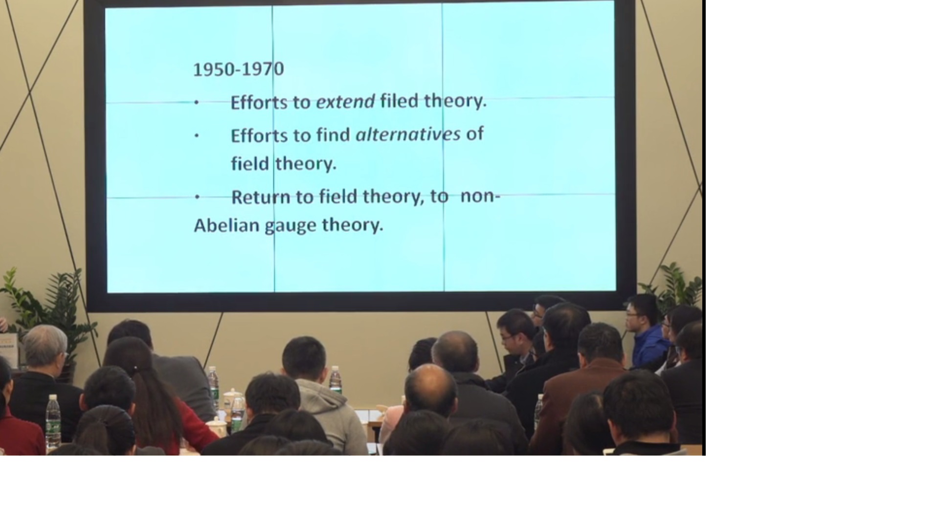
1 引言:量子力学的二元结构和其发展的二元状态

上世纪二十年代, 海森伯(Werner Karl Heisenberg)、薛定谔(Erwin Schrödinger) 和玻恩(Max Born)等人创立了量子力学,奠定了人类认识微观世界的科学基础,直接推动了核能、激光和半导体等现代技术的创新,深刻地变革了人类社会的生活方式。量子力学成功地预言了各种物理效应并解释了诸多方面科学实验,成为当代物质科学发展的基石。然而,作为量子力学核心观念的波函数在实际中的意义如何,自爱因斯坦(Albert Einstein) 和玻尔(Niels Bohr) 旷世之争以来,人们众说纷纭,各执一词,并无共识。可以说,直到今天,量子力学发展还是处在一种令人尴尬的二元状态:在应用方面一路高歌猛进,在基础概念方面却莫衷一是。这种二元状态,看上去十分之不协调。对此有人以玻尔的“互补性”或严肃或诙谐地调侃之,以“shut up and calculate”的工具主义观点处之以举重若轻。

然而,对待量子力学诠释严肃的科学态度应该是首先厘清量子力学诠释中哪一部分观念导致了基本应用方面的“高歌猛进”,哪一部分观念导致了理解诠释方面的“莫衷一是”。对量子力学诠释不分清楚彼此、逻辑上倒因为果的情绪化评价,会在概念上混淆是非,误导量子理论与技术的真正创新。无怪乎,有人以“量子”的名义为认识论中“意识可以脱离物质”的明显错误而张目,其根源就是每个人心目中有不同的量子力学诠释。

我个人认为,这样一个二元状态主要是由于附加在玻恩几率解释之上的“哥本哈根诠释”之独有的部分:外部经典世界存在是诠释量子力学所必需的,是它产生了不服从薛定谔方程幺正演化的波包塌缩,使得量子力学二元化了。今天,虽然波包塌缩概念广被争议,它导致的后选择“技术”却被广泛地应用于量子信息技术的各个方面,如线性光学量子计算和量子离物传态的某些实验演示。

其实,我以上的观点契合了来自一些伟大科学家的伟大声音!现在,让我们再一次倾听来自量子力学创立者薛定谔对哥本哈根诠释直言不讳的批评。早年,薛定谔曾经写信严厉批评了当时的物理学家们,因为在他看来,他们不假思索地接受了哥本哈根解释:“除了很少的例外(比如爱因斯坦和劳厄(Max von Laue)),所有剩下的理论物理学家都是十足的蠢货,而我是唯一一个清醒的人”。薛定谔在写给他老朋友玻恩的一封信中说:

“我确实需要给你彻底洗脑……你轻率地常常宣称哥本哈根解释实际上已经被普遍接受,毫无保留地这样宣称,甚至是在一群外行人面前——他们完全在你的掌握之中。这已经是道德底线了……你真的如此确信人类很快就会屈从于你的愚蠢吗?”

薛定谔传记作者约翰·格里宾(John Gribbin)看到这些信,感叹道:“作为一位在仅仅几年后就接受了哥本哈根解释的教导,并且直到很久之后才意识到这种愚蠢的人,我发现薛定谔在1960 年的这些话直击我心!”

1979 年诺奖得主、物理学标准模型的奠基者之一史蒂文·温伯格(Steven Weinberg)在《爱因斯坦的错误》一文中,很具体、很直接地批评了哥本哈根诠释的倡导者玻尔对于测量过程的不当处理:

“量子经典诠释的玻尔版本有很大的瑕疵,其原因并非爱因斯坦所想象的。哥本哈根诠释试图描述观测(量子系统)所发生的状况,却经典地处理观察者与测量的过程。这种处理方法肯定不对:观察者与他们的仪器也得遵守同样的量子力学规则,正如宇宙的每一个量子系统都必须遵守量子力学规则。”“哥本哈根诠释明显地可以解释量子系统的量子行为,但它并没有达成解释的任务,那就是应用波函数演化确定性方程(薛定谔方程)于观察者和他们的仪器。”

最近温伯格先生又进一步强调了他对“标准”量子力学的种种不满。对哥本哈根诠释的严肃批评自其出笼至今就不绝于耳,但也有不少人却充耳不闻,这显然是一种选择性失聪!在量子信息领域,不少人不加甄别地使用哥本哈根诠释导致的“后选择”方案,其可靠性、安全性必然令人生疑!

其实,在量子力学幺正演化的框架内,多世界诠释不引入任何附加的假设,成功地描述了测量问题,从而对哥本哈根诠释系统而深入的挑战。需要指出的是,此前不久建议的隐变量理论在理论体系上超越了量子力学框架,本质上是比量子力学更基本的理论,因此对此进行检验的Bell 不等式本文不予系统讨论。自上一世纪八十年代初,人们提出了各种看似形式迥异的量子力学诠释,如退相干理论、自洽历史诠释、粗粒化退相干历史和量子达尔文主义。后来经深入研究, 人们意识到,这些诠释大致上是多世界诠释思想的拓展和推广。

2 哥本哈根诠释及其推论

哥本哈根诠释是由玻尔和海森伯等人在1925—1927 年间发展起来的量子力学的一种诠释。它对玻恩所提出的波函数的几率解释进行了超越经典几率诠释的推广,突出强调了波粒二象性和不确定性原理。虽然人们心目中量子力学哥本哈根诠释有各种各样版本,但对其核心内容人们还是有所共识的,那就是“诠释量子世界,外部的经典世界必不可少”。

大家知道,微观世界运动基本规律服从薛定谔方程,可以用演化波函数描述;等效地,也可以用涉及不可对易力学量的运动方程和系统定态波函数。这两种运动方程描述都保证了波函数服从态叠加原理:如果|ϕ1> 和|ϕ2> 满足运动方程,则

也是微观世界满足运动方程的可能状态。当|ϕ1> 和|ϕ2> 是某一个力学量的本征态(对应本征值a1和a2),则根据玻恩几率解释,对|ϕ> 测量A 的可能值只能随机地得到a1和a2,相应的几率是|c1|2 和|c2|2 。因而,A平均值是

这就是玻恩几率解释的全部内容,不必附加任何假设,足以用它理解微观世界迄今为止所有的实验数据。

结合量子力学的数学框架中波函数假设和基本运动方程,玻恩几率解释构成了量子力学的基本内容,可以正确预言从基本粒子到宏观固体的诸多物理特性和效应。但哥本哈根诠释却要通过附加的假设拓展玻恩几率解释。这个拓展从冯·诺依曼(John von Neumann)开始,追问测量后的波函数是什么。这个追问满足了人们对终极问题的刨根问底,同时物理上的诉求也是合情合理的,即,对紧接着的重复测量测后系统给出相同的结果。

冯·诺依曼首先把测量定义为相互作用产生的仪器(D)和系统(S)的关联(也可以笼统地叫做纠缠)。特殊相互作用导致的总系统D+S 演化波函数为

根据上面的方程,一旦观察者发现了仪器在具有特制经典的态|D1> 上, 则整个波函数塌缩到|ϕ1>⊗ |D1> ,从而由仪器状态D1 读出系统状态|ϕ1> ,对|ϕ2> 亦然。自此,哥本哈根学派或与有关人士把这种波包塌缩现象简化为一个不能由薛定谔方程描述的非幺正过程:在|ϕ> 上测A,测量一旦得到结果a1,则测量后的波函数变为|ϕ> 的一个分支|ϕ1> 。这个假设的确保证了紧接着的重复测量给出相同的结果。

然而,玻尔从来都不满足于物理层面上的直观描述和数学上的严谨表达,对于类似波包塌缩的神秘行为他进行了“哲学”高度的提升:只有外部经典世界的存在,才能引起波包塌缩这种非幺正变化,外部经典世界是诠释量子力学所必不可少的。

加上波包塌缩假设,人们把量子力学诠释归纳为以下6条:

(1)量子系统的状态用满足薛定谔方程的波函数来描述,它代表一个观察者对于量子系统所能知道的全部知识(薛定谔);

(2)量子力学对微观的描述本质上是概率性的,一个事件发生的概率是其对应的波函数分量的绝对值平方(玻恩);

(3)力学量用满足一定对易关系的算符描述,它导致不确定性原理:一个量子粒子的位置和动量无法同时被准确测量(海森伯), ΔxΔp ≥ℏ/2;

(4)互补原理(Complementarity principle,亦译为并协原理):物质具有波粒二象性,一个实验可以展现物质的粒子行为或波动行为,但二者不能同时出现(玻尔);

(5)对应原理:大尺度宏观体系的量子行为接近经典行为(玻尔);

(6)外部经典世界是诠释量子力学所必需的,测量仪器必须是经典的(玻尔与海森伯)。

一般说来,“哥本哈根诠释”特指上述6 条量子力学基本原理中的后4 条。然而,玻尔等提出的4 条“军规”,看似语出惊人,实质却可证明为前两条的演绎。第3 条海森伯不确定性关系并不独立于玻恩几率解释。只是由于不确定关系能够凸显量子力学的基本特性——不能同时用坐标和动量定义微观粒子轨道,看上去立意高远!玻尔和海森伯等从哲学的高度把它提升到量子力学的核心地位。但是,今天大家意识到,只要用波函数玻恩解释给出力学量平均值公式,就可以严格导出不确定关系。其实,在研究具体问题时,不确定性关系可以解释一些新奇的量子效应,但不能指望它给出所有精准的定量预言。

哥本哈根“军规”第4 条——玻尔互补原理后半句话“波动性和粒子性在同一个实验中,二者互相排斥、不可同时出现”经常被人们忽略,但它却是互补原理的精髓所在。玻尔互补原理在一定的意义上可以视为哲学性的描述。玻尔本人甚至认为可以推广到心理学乃至社会学,以彰显其普遍性!然而,虽然它看似寓意深奥,在操作层面上却不完全独立于不确定性关系。量子力学的奠基者之一、也被视为哥本哈根学派主力的保罗·狄拉克(Paul Dirac)对此有不屑的态度。对于玻尔那种主要表现在互补原理之中的“啰嗦的、朦胧的”哲学,狄拉克根本无法习惯。1963年,狄拉克谈到互补原理时说,“我一点也不喜欢它”,“ 它没有给你提供任何以前没有的公式”。狄拉克不喜欢这个原理的充分理由,从侧面反映了互补原理不是一般的可以用数学准确表达的物理学结论。其实,尽管互补原理不能吸引狄拉克,但也许还是潜移默化地影响了他的思维,在狄拉克《量子力学原理》前言当中及其他地方,他强调的不变变换可以看做是玻尔互补观念的一种表现。

其实,我们能够清晰地展示互补原理的不独立性。在粒子双缝干涉实验中,要探知粒子路径意味着实验强调粒子性,波动性自然消失,干涉条纹也随之消失,发生了退相干。玻尔互补原理对此进行了哲学高度的诠释:谈论粒子走哪一条缝,是在强调粒子性,因为只有粒子才有位置描述;强调粒子性,波动性消失了,随即也就退相干了。海森伯用自己的不确定性关系对这种退相干现象给出了比较物理的解释:探测粒子经过哪一条缝,相当于对粒子的位置进行精确测量,从而对粒子的动量产生很大的扰动,而动量联系于粒子物质波的波矢或波长,从而导致干涉条纹消失。海森伯本人认为,通过不确定性关系很好地印证了互补性原理。然而,玻尔并不买海森伯的帐,认为只有互补原理才是观察引起退相干问题的核心,测量装置的预先设置决定了“看到”的结果。强调不确定性关系推导出互补性,本质上降低了理论的高度和深度。当然,玻尔本人也认为不确定性关系是波粒二象性的很好展现: Δx很小,意味着位置确定,这对应着粒子性,这时Δp 很大,波矢不确定所以波动性消失了。哥本哈根“军规”第5 条是对应原理,它可以视为薛定谔方程半经典近似的结果。

经过这样的分析甄别,可以断定只有第6 条才是“哥本哈根诠释”独特且独立的部分,也正是它导致了量子力学诠释的二元论结构:微观系统服从导致幺正演化的薛定谔方程(U 过程),但对微观系统测量过程的描述则必须借助于经典世界,它导致非幺正的突变(R 过程)。罗杰·彭罗斯(Roger Penrose)多次强调,量子力学哥本哈根诠释的全部奥秘在于量子力学是否存在薛定谔方程U过程以外的R过程。

当年,玻尔认为这种描述是十分自然的:为了获取原子微观世界的知识,对于生活在经典世界的人类而言,所用的仪器必须是经典的。然而,仪器本身是由微观系统组成,每一个粒子服从量子力学,经典与量子之间必存在边界,但边界却是模糊的。哥本哈根诠释要想自洽,就要根据实际需要调整边界的位置,可以在仪器—系统之间,可以在仪器—人类观察者之间,甚至可以是视觉神经和人脑之间。

如果说“边界可变”的哥本哈根诠释是一条灵动而有毒的“蛇”,哥本哈根“军规”第6 条是其最核心、最致命的地方。温伯格先生对此的严厉批评和质疑,正好打了“蛇”的七寸。七寸处之“毒”在意识论上会导致冯·诺依曼链佯谬:人的意识导致最终波包塌缩。让我们考察冯·诺依曼量子测量的引申。我们不妨先承认玻尔的“经典必要性”。如果第一个仪器用量子态描述,为什么系统+仪器的复合态会塌缩到|ϕ1>⊗|D1> ,答案自然是有第二个经典仪器D2 存在,使得更大的总系统塌缩到|ϕ1>⊗|D1>⊗|D2> ⋯ 。以此类推要塌缩到以下链式分支上:

据此类推,最末端的仪器在哪里呢?那么,要想有终极的塌缩, 末端必须是非物质“ 神” 或“人”的意识。冯·诺依曼的好友维格纳(Eugene Wigner)就是这样推断意识会进入物质世界。

我个人猜想,目前国内有人由量子力学论及“意识可独立于物质而存在”,正是拾维格纳的牙慧,把哥本哈根诠释进行这种不合理的逻辑外推。然而,这个结论逻辑上是有问题的,如果我们研究的系统是整个宇宙,难道有宇宙之外的上帝?对此的正确分析可能要涉及一个深刻的数学理论:随着仪器不断增加到无穷,我们就涉及了无穷重的希尔伯特空间的直积。无穷重和有限重直积空间有本质差别,序参量出现就源于此。

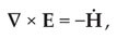
哥本哈根诠释还有一个会引起歧义的地方:波包塌缩与狭义相对论有表现上的冲突。例如,如图1,一个粒子在t=0 时刻局域在一个空间点A上,t=T 时测量其动量得到确定的动量p,则波包塌缩为动量本征态φ(x)~ exp( ipx) ,其空间分布在T 时刻后不再定域,整个空间均匀分布。因此,测量引起的波包塌缩导致了某种定域性的整体破坏:虽然B 点在过A 点的光锥之外(即A 和B 两点是类空的,通常不存在因果关系),但在t >T的时刻,我们仍有可能在B 点发现粒子。按照狭义相对论,信号最多是以光的速度传播,而在瞬时的间隔发生的波包塌缩现象,意味着存在“概率意义”的超光速——T 时刻测量粒子动量会导致体系以一定几率(通常很小很小) “ 超光速”地塌缩到不同的动量本征态上。这个例子表明,如果简单地相信波包塌缩是一个基本原理,会出现与狭义相对论矛盾的悖论。事实上,对于单一的测量,我们并不能确定地在B点发现粒子。因此,“事件”A和B的联系只是概率性的。而对于微观粒子而言,讨论经典意义下的因果关系和相关的非定域性问题,不是一个恰当的论题。概率性的“超光速”现象意味着,在概率中因果关系必须要仔细考量。

图1 四维时空中的整体波包塌缩:对定域态的动量测量,接受哥本哈根的观点,则会认为系统塌缩到动量本征态,从而可以出现在类空点上

综上所述,哥本哈根诠释带来概念困难的关键之处是广为大家质疑的第6 条“军规”——经典必要性或波包塌缩。量子力学的其他诠释,如多世界诠释、退相干诠释乃至隐变量理论,均是针对这一点,提出了或是在量子力学框架之内、或是超越之外的解决方案。

3 多世界诠释

对量子力学诠释采取“工具论(instrumentalism)”的态度,可以认为波函数不代表任何物理世界中的实体,也不描写实际的测量过程,而只是推断实验结果的数学工具。因此,在哥本哈根诠释中,波包塌缩与否,都不意味着实体塌缩,只是塌缩后可以据此推断重复测量的结果。虽然玻尔自己晚期也多次谈到这一点,但哥本哈根学派的思想并没有逻辑上的一致性。他们由此推及诠释量子力学必须借助经典世界,明显走向了本体论(ontology)的一面,经典世界是客观存在的本体。因此,从哲学意义上讲,哥本哈根诠释是一种二元论的混合体:微观世界由观察或意识决定,但实施观察的经典世界是客观存在的。

温伯格和盖尔曼(Murray Gell-Mann)等著名的理论物理学家,并不满足于哥本哈根诠释的绥靖主义和哲学上二元论的理解,他们从实在论(realism)立场出发,直到今天还在锲而不舍地追问波函数到底是什么、测量后变为什么。非常幸运,早在上一个世纪五十年代初,埃弗里特对这些基本问题给出了“实在论”或“本体论”式的回答——这就是相对态理论或后称多世界诠释。

量子力学的多世界诠释起源于休·埃弗里特(Hugh Everett)(图2)的博士论文。1957 年在《现代物理评论》发表了这个博士论文的简化版。发表文章的题目《量子力学的相对态表述》有些专业化,但科学上很准确。文章发表后被学界冷落多年,1960 年代末德维特(Bryce Seligman DeWitt)在研究量子宇宙学问题时,重新发现了这个“世界上保守好的秘密”,并把它重新命名为“多世界理论”。这个引人注目的名称复活了埃弗里特沉寂多年的观念,也引起了诸多新的误解和争论。

图2 休·埃弗里特(1930—1982):多世界诠释的创立者

埃弗里特提出多世界诠释之后,面对玻尔的冷落,不管他的老师惠勒(John Wheeler)如何沟通“多世界理论”和“标准”哥本哈根诠释、平滑它们的冲突,在答复《现代物理评论》编辑部的批评意见时,他还是挑明了他与哥本哈根诠释的根本分歧。他认为:“哥本哈根诠释的不完整性是无可救药的,因为它先验地依赖于经典物理……这是一个将‘真实’概念建立在宏观世界、否认微观世界真实性的哲学怪态。”这一点也是温伯格在尖锐批评哥本哈根诠释时所不断重复的要点、灵动之“蛇”的七寸。今天,不少人认为,多世界诠释的建立是使量子力学摆脱“怪态”走向正常态的基本理论。

多世界诠释认为,微观世界中的量子态是不能孤立存在的,它必须相对于它外部一切,包括仪器、观察者乃至环境中各种要素。因此,微观系统不同分支量子态|n> 也必须相对于仪器状态|Dn> ,观察者的状态|On> ……环境的状态|En> 来定义,从而,微观系统状态嵌入到一个所谓的世界波函数或称宇宙波函数(universal wavefunction):

它是所有分支波函数的叠加。埃弗里特等人认为,如果考虑全了整个世界的各个部分细节,Cn可以对应于微正则系综Cn = 1/√N,N 是宇宙所有微观状态数。不必预先假设玻恩规则,通过粗粒化,可以证明|Cn|2 代表事件n 发生的概率。当然,这种处理取决于人们对概率起因的理解。

图3 薛定谔猫“佯谬”多世界图像:处在基态|0> 和激发态|1> 叠加态上的放射性核,通过某种装置与猫发生相互作用。处在|1> 态的核会辐射,触动某种装置杀死猫,而处在|0> 态的核不辐射,猫活着。这个相互作用结果使得世界处在两个分支上:在“死猫”的分支上,核辐射了,杀死了猫,观察者悲伤,也看到了这个结果,整个世界也为之动容;在“活猫”分支上,没有辐射,没有猫死,没有悲伤的观察者和悲切的世界。两个分支都存在,但观察者们不会互知彼此

多世界诠释认为,量子测量过程是相互作用导致了世界波函数的幺正演化过程,测量结果就存在于它的某一个分支之中。每一个分支都是“真实”存在,只是作为观察者“你”、“我”恰好处在那个分支中。薛定谔猫在死(活)态上,对应着放射性的核处在激发态|1> (基态|0> )上,这时观察者观测到了猫是死(活)的。我们写下猫态:

多世界诠释是说, 两个分支|-> =|死,1,O1> ≡ |死>⊗|1>⊗|O1> 和|+> = |活,0,O0>≡ |活>⊗|0>⊗|O0> 都是真实存在的。测量得到某种结果,如猫还活着,只是因为观察者恰好处在|+> 这个分支中。

如果仅仅到此为止,人们会马上质疑多世界理论,并视之为形而上学:仅说碰巧观察者待在一个分支内,作为观察者的“你”、“我”在另一个分支里看到了不同的结果,观察者的“你”、“我”便“一分为二”了。人们显然不会接受这种荒诞的世界观。然而,埃弗里特、德维特利用不附加任何假设的量子力学理论,自洽地说明不同分支之间,不能交流任何信息。因此,在不同分支内,观察者“看到”的结果是唯一的。最近,本文作者及合作者通过明确定义什么是客观的量子测量,严格地证明了这个结论。我们的研究进一步表明,埃弗里特的多世界诠释变成了一个犹如量子色动力学(QCD)一样正确的物理理论。QCD假设了夸克,但“实验观察”并没有直接看到夸克的存在。所幸QCD本身预言了渐进自由,它意味着夸克可能发生禁闭:两个夸克离得越近,它们相互作用越弱,反之在一定程度上,距离越远,相互作用越强,因而不存在自由夸克(当然,严格地讲,渐进自由是依据微扰QED证明的,而QCD 研究禁闭问题的本质可能是非微扰)。

多世界理论常常被误解为假设了世界的“分裂”、替代波包塌缩。事实上,埃弗里特从来没有做过这样的假设。多世界理论是在量子力学的基本框架(薛定谔方程或海森伯方程加上玻恩几率诠释)描述测量或观察,不附加任何假设。“分裂”只是理论中间产物的形象比喻。当初,埃弗里特投稿《现代物理评论》遭到了审稿人的严厉批评:测量导致的分支状态共存,意味着世界在多次“观测”中不断地分裂,但没有任何观察者在实际中感受到各个分支的共存。埃弗里特对这个问题的答辩也是思辨式的,但逻辑上很有说服力。他说,哥白尼的日心说预言了地球是运动的,但地球上的人的经验从来没有直接感觉到地球是运动的。不过,从日心说发展出来的完整理论——牛顿力学从相对运动的观点解释了地球上的人为什么会感觉到地球不动。理论本身可以解释理论预言与经验的表观矛盾,这一点正是成功理论的深邃和精妙所在。

今天看来,作为理论中间的要素,不自由的夸克和不可观测的世界分裂都是一样的“ 真实”,其关键是量子力学的多世界诠释能否自证“世界分裂”的不可观测性。由于世界波函数的描述原则上包含了所有的观察者,上帝也不可置身此外。因此,我们不再区分仪器、观察者或上帝,世界是否“分裂”问题于是就转化为观察或测量的客观性问题(Box 1):两个不同观察者观察的结果是否一致,观测结果之间是否互相验证一致。

事实上,为了证明多世界诠释中世界的分裂是不可观测的,埃弗里特首先明确什么是“观察”或“测量”。今天大家已经公认,测量是系统和仪器之间的经典关联,如果要求这种关联是理想的,对应于不同系统分支态的仪器态是正交的(完全可以区分)。如果观察者可以用另外的仪器去测量原来的仪器状态,得到相同的对应读数, 则两个仪器间形成理想的经典关联(Box 1)。

多世界诠释似乎完美地解决了哥本哈根诠释中面临的关键问题,但其自身仍然在逻辑上存在漏洞,这就是偏好基矢(preferred basis)问题。我们以自旋测量为例说明这个问题,设自旋1/2 体系世界波函数为

其中|U↑>(|U↓> ) 代表相对于自旋态|↑> (|↓>) 的宇宙其他所有部分的态。按多世界论的观点,测得了自旋向上态|↑> , 是因为它的相对态|U↑> = |D↑,O↑,⋯> 包含了指针向上的仪器D↑ ,看到这个现象观察者O↑ 以及相应的环境等。多世界诠释的要点是认为另外一个分支|U↓> =| D↓,O↓,⋯> 仍然是“真实”存在,但外在另一个(向上)分支中的观察者无法与这个分支进行通信,不能感受到向下分支的存在。然而,量子态|ϕ> 的表达式不唯一,即原来的世界波函数也可以表达为

其中新的基矢|±> = (|↑> ± |↓> )/√2 代表自旋向左或向右的态,而|U±> = (|U↑> ± |U↓> )/√2 代表系统与世界相对应的部分。很显然, |U±> 不会简单地写成仪器和观察者因子化形式,它不再是仪器、观察者和环境其他部分的简单乘积,测量的客观性不能得以保证。

上述考虑带来了所谓的偏好基矢问题:为什么对于同一个态,在谈论自旋取向测量时,我们采用了自旋向上和向下( |↑> 和|↓> )这种偏好,而非自旋左右。埃弗里特知道这个问题的存在,但他并不在意,他觉得任何测量都要有体现功能的仪器的特定设置,这种功能选择设置仪确定了偏好基矢。例如,在测量自旋的施特恩—盖拉赫实验中,我们通过选择非均匀外磁场的指向,来确定是测上下还是左右的自旋。然而,很多理论物理学家还是觉得多世界理论的确存在这样的不足。1981 年祖莱克(Wojciech Zurek)把迪特尔·泽(Dieter Zeh)1970 年提出的量子退相干观念应用到量子测量或多世界理论,为解决偏好基矢问题开辟了一个新的研究方向。

Box1:“世界分裂”的不可观察(测量)性

我们先假设观察者O通过仪器D测量系统S。三者的相互作用导致系统演化到一个我们称之为世界波函数的纠缠态:

在每一个分支中, {|S>} 是系统的完备的基矢, {|dS>} 和{|OS>} 分别是与系统基矢|S> 相对应的仪器和观察者的态基矢。为了简单起见,一般情况下|OS> 可以代表系统和仪器以外世界所有部分,包括观察者和整个环境,通常不预先要求它们是正交的。

由于O是宏观的,则它对量子态反映是敏感的,有<OS|OS′> = δSS′。平均掉环境作用,系统和仪器之间形成一个经典关联,

进而,如果仪器态是正交的, <dS|dS′> = δSS′ ,则ρSD 代表一种理想的经典关联。这时,如果观测的对象是系统的力学量A, |S> 是它的本征态, A|S> = aS|S> ,则系统本征态是正交的,从而仪器和观察者之间也形成理想的经典关联:

这表明,观察者O在仪器D上读出了S,且对于aS的几率为|CS|2 。

以上分析表明,观察者O用仪器D测量系统S 的(厄米)力学量A,理想的测量要求三体相互作用导致的纠缠态|φ> 是一个GHZ 型态,即 {|dS>} 和{|OS>} 是两个正交集。这时,观察者和系统之间也会形成一个系数相同的理想经典关联态,

因而我们说测量是客观的,这里可以把仪器和观察者当做两个不同的观察者,不同的观察者看到相同的结果。

现在我们假设仪器的状态 |dS>不是正交的,则|dS>可以用正交基|DS> (B|DS> = dS|DS>) 展开:

其中, CSS′= <DS′|dS> 。这时

这表明|S> 分支中的观察者有一定的几率看到了另一个分支中仪器的读数——分支态|Dm> ,观察到了“分裂”!因此,要求理想测量( |φ> 是理想的GHZ态),则我们观测不到分裂。

我们还可以用反证法说明世界分裂是不可观察的。设世界波函数为

当|O1> = |O2> ,观察者O不能区分|S1> 和|S2> ,因此看到了世界的分裂,或

代表着观察者O看到世界分裂,因为它不能区分|S1> 和|S2> 。这时,

非对角项的存在意味着仪器和系统之间不能形成很好的经典关联。

4 量子退相干诠释或理论

提出量子退相干观念的目标之一是要解决所谓的“薛定谔猫佯谬”,即为什么常态下宏观物体不会展现量子相干性。大家知道,接着波粒二象性的观点,任何实物粒子可以表现出波动行为,可以发生低能物体穿透势垒的量子隧道效应。关于微观体系,电子、原子、中子、准粒子(库珀对)乃至C60这样的大分子,实验上已经展示了量子隧道效应,并在实际技术中得到了广泛应

用,如STM(扫描隧道显微镜)。现在的问题是一个宏观物体,像足球、人、崂山道士,可否发生量子隧道效应?崂山道士可否破墙而出,破墙而入?初步的看法是,这是不可能的,因为宏观物体的质量较大,物质波波长短,必远远小于物体的尺度,不可能展示出量子相干效应。

迪特尔·泽和他的学生埃里希·朱斯(Erich Joos)(图4)从另一个角度给出了相同的答案:一个宏观物体必定和外部环境相互作用,即使组成环境的单个微粒很小,与宏观物理碰撞时能量交换可以忽略不计,环境也可以记录宏观物体运动信息,从而与宏观物体形成量子纠缠,发生量子退相干。此时,环境的作用相当于在系统不同基矢态中引入随机的相对相位,平均结果使得干涉项消失。因此,不同的(动量)态之间的相干叠加不存在了。

图4 量子退相干理论创立者迪特尔·泽(左图,http://www.ijqf.org/members-2/dieter/)和他的学生埃里希·朱斯(右图)

量子退相干理论最近已引起物理学界极度重视,一个重要原因是量子通讯和量子计算研究的兴起。量子计算利用量子相干性——量子并行和量子纠缠以增强计算能力,而退相干对其物理实现造成了巨大障碍。当年迪特尔·泽提出量子退相干的概念时只是一位讲师,他的文章不能在知名的学术刊物上发表,创新的观点受到著名学者尖酸的批评,整个70 年代这个重要工作被物理学家系统性忽视,几乎影响了迪特尔·泽后来的学术职业生涯。后来,退相干理论渡过1980 年代这个黑暗期,祖莱克加入量子退相干研究队伍。他的着眼点是解决偏好基矢问题,并为量子测量问题的探索提供了新的思路。

在量子退相干理论中, 处在初态|φS&gt; =ΣCn|n&gt; 的系统与处在初态|E&gt; 上的环境发生非破坏(不交换能量)的相互作用,使得t 时刻总的状态变为

这里|En(t)&gt; =Un(t)|E&gt; ,而Un = exp(-iHnt )是非破坏相互作用V =Σ|n&gt;&lt;n|Hn中分支哈密顿量Hn决定的时间演化。这时,体系的约化密度矩阵

一般包含非对角项,其中Fmn= &lt;Em| En&gt; 称为退相干因子。当Fmn = 0 ,则非对角项消逝,即

这时,描述大系统量子态的量子相干叠加态|φS&gt;变成了没有量子相干的密度矩阵,实现了从量子叠加态到经典几率描述的转变。这相当于实空间中干涉条纹消逝(Box2)。

Box 2:量子干涉与量子退相干

为了考察量子相干性与通常量子干涉之间的关系,我们在坐标表象{φ(x) = &lt;x|φ&gt;,φn(x) = &lt;x|n&gt;} 中写下密度分布:

其中ρd(x) =Σ|Cn|2|φn(x)|2代表强度相加项, 而Σn≠mCm*CnFmn(t)φm*(x)φn(x) 代表相干条纹,当Fmn(t) = 0 相干条纹消逝。

我们从双缝实验可以进一步形象地说明这一点。由中子源出射的中子束经双缝在屏S上干涉。

遮蔽上( 下) 缝的波函数|0&gt; (|1&gt;) 的坐标表示为

φu(x) = &lt;x|0&gt; ∝ eikx(φd(x) = &lt;x|1&gt; ∝ eik(x + Δ)), 其中Δ = ld- lu是“光程差”。于是, |φ&gt; ∝ |0&gt; + |1&gt; 给出约化密度矩阵:

当&lt;E0| E1&gt; = 1 ,则ρ(x)∝ cos Δk ,否则ρ(x) = 常数,无干涉条纹。

综上所述,环境的存在就像一个观察者在不断地监视着系统的运动,它通过与系统纠缠引入了等效的随机相位Δθ , 状态|φ(0)&gt; = |0&gt; + |1&gt; , 被测后变为|φ′&gt; = |0&gt; + eiΔθ|1&gt; ,平均结果给出:

其中,随机相位Δθ 是由等效相位因子eiΔθ的平均值&lt;eiΔθ&gt; = &lt;E0| E1&gt; 来定义。当它趋近于零,干涉条纹消逝,即退相干发生。

我们的研究证明,即使宏观物体与外界完全隔离,内部自由度与质心运动自由度的耦合也会引起退相干,特别是当环境是由很多粒子组成,则可能有因子化的末态|En&gt; =Πj=1N|en(j)&gt; ,它给出退相干因子F01= &lt;E0| E1&gt; =Πj=1N&lt;e0(j)|e1(j)&gt; 。由于|&lt;e0(j)|e1(j)&gt;| &lt; 1 ,当N → ∞ , F01→ 0 ,这个发现原则上解决了薛定谔猫佯谬。只许把“ 死” 与“活”当成质心自由度的状态,完整的猫态应当写为

则猫的密度矩阵的非对角项|死&gt;&lt;活|将伴随着退相干因子FDL =Πj=1N&lt;dj|lj&gt; 。显然,宏观猫的干涉项正比于FDL,在宏观极限下, N → ∞ , FDL= 0 ,从而干涉效应消逝。

针对各种实际中的宏观粒子,迪特尔·泽和他的学生埃里希·朱斯在1985 年仔细地计算了它们在各种环境中空间运动的退相干因子。他们得到一般的系统约化的密度矩阵:

其中局域化因子

决定于环境粒子在宏观物体上的有效散射界面σeff 。表1给出了各种物体局域化因子的列表。

表1 各种物体的局域化因子

总之,作为客观物体象征的薛定谔猫或仪器的运动,可分为集体运动模式和内部相对运动模式,它们之间存在某种形式的信息交换,但不交换能量,由于这种特殊形式的耦合,形成集体运动模式和内部相对运动模式的量子纠缠,内部运动模式提供了一种宏观环境。如果观察者只关心集体运动而不关心内部细节,集体运动就会发生量子退相干,薛定谔猫佯谬也就不存在了。

我们最近发现,薛定谔猫的退相干还有一个内禀的原因,这就是相对论效应:一群自由粒子,其能量最低阶非相对论效应正比于p4,它使得质心自由度与内部自由度内禀地耦合起来,产生薛定谔猫的内禀退相干。这个发现进一步表明,“月亮”在没有人看它的时候,仍然是客观存在的。这是因为“月亮”是一个宏观物体,人类的“看”必定忽略了“月亮”的内部细节。由于相对论效应,内部环境与“看到”的宏观自由度有天然的耦合,使得退相干无处不在!

以上的分析可以正面回答目前热炒的“量子意识”问题。我们认为,把至今备受质疑的哥本哈根诠释的波包塌缩假设作为论证基础,大谈量子意识,科学知识非常之不准确!虽然现在的物理理论还不能完全解释意识,但也绝不能断言它与量子有直接关系。因为意识必源自人这样的常态宏观物体,后者注定退相干。把量子力学和意识这种高级生命独有的现象联系起来并没有为理解意识的产生与存在提供任何高于猜测的理解。其实,物理学解释不了的问题就不应该牵强附会地解释。要承认科学的定位和局限性,有些问题不在目前科学研究范畴内,非要披上科学的外衣就是对科学的侵犯。

1981 年,祖莱克(图5)把迪特尔·泽的量子退相干理论应用到冯·诺依曼量子测量理论,把测量过程看成系统S 与测量仪器D相互作用产生经典关联的一种动力学过程。在冯·诺依曼量子测量中,通过与环境作用,系统+仪器形成的复合系统进一步与环境量子纠缠:

从而有复合系统的约化密度矩阵变为

现在,相互作用只是产生系统态|n&gt; 与仪器态|Dn&gt;的量子纠缠,并非纯概率性的关联。当其中退相干因子Fmn= &lt;En| Em&gt; → 0 时, ρSD→Σ|Cn|2|n,Dn&gt;&lt;n,Dn| ,退相干后的约化密度矩阵代表了关联是以经典几率的方式出现。就像天气预报,明天下雨的几率为30%,不下雨几率为70%,是一种经典随机现象,没有任何量子相干效应。测量就是这样一个产生关联的过程,而无须什么波包塌缩!

图5 祖莱克(Wojciech Zurek,全海涛2006 年摄影)

需要强调的是,应用于量子测量问题,退相干理论必须能够解释指针态(pointer state)的衍生(emergence)。这个概念与多世界理论中相对态的观念是一致的。如上所述,环境作用选择仪器+系统的特定基矢进行退相干,而密度矩阵的对角元和非对角元则在不同的坐标变换下是相对的。如果采用另一组基矢|n′&gt; =ΣSnn′+|n&gt;,则有非对角项|n′&gt;&lt; m′| 的存在。正是由于这种基矢的相对性,量子纠缠无法直接描述量子测量,这就是所谓的偏好基矢问题。

在整个宇宙(系统+仪器+外部环境)的时间演化过程中,因子化的宇宙初态会变成一个针对被测基矢的相对态,相对态中每一项的系数恰好是初态中系统相干叠加态中的系数。这时,我们说相对系统态而言,仪器态是一个指针态,而环境所充当的角色是诱导了一个超选择定则(称为eniselection),选择了这样特定的基矢。退相干理论的第二个要点是初态因子化的假设。它隐含的意思是,没发生相互作用之前,系统的相干叠加态是独立于测量仪器和环境而存在的。以后,相互作用使得世界波函数保持一种准因子化的形式,即形成具有和系统初态系数一样的施密特系数的相对态。这个假设可以有一个逻辑上的改进。因为因子化形式依赖于张量积定义,其不唯一性使退相干理论进一步也遭遇到质疑的逻辑障碍。也许这与偏好基矢问题是等价的。在更完美的理论中,应该事先不假定因子化的形式,让环境诱导出来的时间演化产生相对态的系数,实现完全客观的量子测量过程。但是,这种处理遇到的关键问题是怎样把这个理论结果与依赖于初态的实验相比较。

5 量子自洽历史、量子达尔文和各种诠释的统一

量子退相干理论强调的是环境引起的量子退相干,但对于整个宇宙而言,谈其环境是没有意义的,宇宙本质是个孤立体系。如果有朝一日人们完成了引力量子化,没有环境影响,经典引力如何出现?没有经典引力,我们如何理解苹果落地和月球绕日而行、如何描述整个宇宙在经典引力作用下的演化?因此,为了描述量子宇宙的所有物理过程,我们的确需要一个更加普遍的量子力学诠释:这里没有外部测量,也没有外部环境,一切都在宇宙内部衍生,在宇宙内部也可以看到一个从量子化宇宙约化出来的经典世界,经典引力支配着各种各样的物理现象。针对这个问题,基于格里菲斯(Robert Griffiths)和欧内斯(Roland Omnes)等人提出自洽历史处理(consistent history approach),哈特尔(James B. Hartle)和盖尔曼等人发展了退相干历史的量子力学诠释。

量子力学自洽历史诠释是格里菲斯(图6)在1983 年提出来的。与多世界诠释一样,量子力学自洽历史诠释也是从世界波函数出发,它强调的“历史”是有测量介入的离散时间演化序列。如图7,我们用一个描述测量结果的投影算符序列

来定义量子世界包含时间演化和测量的历史。Pj代表在t=j 时到某本征态上的投影。不同的历史,相当于多世界理论中世界分裂的不同分支。显然,任意给定一个历史的集合,不同的历史之间有干涉效应,每一个历史相互不“独立”,不能定义经典几率。为了衍生出经典概率,格里菲斯对描述历史的投影算符乘积给出了自洽条件Tr(HjρHl)= 0( j ≠ l) ,其中ρ 代表系统的密度矩阵。满足这个条件的历史集合中的历史被称为自洽的历史。对每一组自洽的历史,可以赋予一个经典概率描述: Pr( j) = Tr(HjρHj) 。如果把每一个历史当成多世界理论中世界波函数时间域上的一个分支,自洽历史处理可以视为多世界理论的某种推广发展。在这个意义下,多世界可以看成是我们唯一宇宙“多种选择的历史”。按美国加州理工学院的哈特尔和盖尔曼的观点,虽然世界只有一个,但却可以经历很多个可能历史组。

图6 自洽历史诠释的创立者格里菲斯(Robert Griffiths,孙昌璞2005 年摄影)

图7 自洽历史诠释与多世界理论的相似性:“世界只有一个,历史是多重的”

下面以薛定谔猫佯谬为例,简要地告诉大家什么是自洽历史描述:如果我们能够测量每一个时刻组成猫的所有粒子的坐标,不同时刻的位置测量构成了系统的精(细)粒化的历史。不同时刻的位置投影算子乘积Hi=Πt=1TΠ(t) 构成历史的描述,其中

指标j 代表组成猫的不同粒子。Hi =H(t = 0,1,,T ) 描述了粒子的轨迹,不同Hi可能会不“独立”,这样历史通常是不自洽的。我们猜想,对于薛定谔猫而言,描述质心运动的那些投影Hi,忽略量子涨落,艾伦菲斯特方程退化成牛顿方程,形成一组自洽的历史,然后赋予经典意义上的几率。我们猜想,只对应轨迹退相干的投影乘积序列,才可以确定地构成自洽的历史。因此,自洽历史诠释的坐标表示本质上是退相干历史诠释。

哈特尔和盖尔曼等人发现,带有测量的历史序列可以用路径积分表达。针对量子引力和宇宙学,提出今称为退相干历史的量子力学诠释:宇宙体系演化过程粗粒化抹除若干可观察对象类之间的量子相干性,经典几率可以自洽地赋予每一个可能的路径。事实上,对任何瞬间宇宙中发生的事件作精确化的描述,构成了一个完全精粒化历史(completely fine-grained history)。不同精粒化的历史之间是相互干涉的,不能用独立的经典概率加以描述。但是,由于宇宙内部的观察者能力的局限性或需求的不同,只能用简化的图像描述宇宙(如只用粒子的质心动量和坐标刻画粒子的运动),本质上是对大量精粒化历史进行分类的粗粒化(coarse-grained)描述。粗粒类内的相位无规可以抹除各类粗粒化历史之间的相干性,从而使得粗粒化的历史形成所谓退相干的历史(decoherence history)。通过这种退相干历史的描述,原则上对量子引力到经典引力的约化给出了自恰的描述。

我们还可以借助“薛定谔猫”来展示什么是退相干历史诠释。假设“猫”作为一个宏观物体是由大量有空间自由度的粒子组成,每一个粒子有自己空间运动的轨迹,满足各自的薛定谔方程,它们每一个的演化构成了“猫”的精粒化的历史,代表了“猫”的动力学所有的微观态细节。如果用路径积分描述这些“历史”,则不同路径之间是干涉的。由于这些粒子间存在相互作用,则“精粒化历史”对应的“轨道”与自由粒子的轨道不是一一对应的。现在我们不关心组成“猫”的每一个粒子的运动细节,只关心它的质心或者其他宏观自由度。某个特定宏观自由度的运动是微观自由度某种集体合作的结果,可以视为“猫”的所有微观演化过程的粗粒化。由于相对运动的影响,它的相干叠加态的时间演化会导致相位差的不确定性,从而相干性消逝。如图8所示,从路径积分的观点看,粗粒化后两条不同路径是不相干的,相干函数变为零,从而导致所谓退相干的历史。

图8 粗粒化导致观察结果的量子退相干:从轨道到轨道类的路径积分

不管退相干历史也好,自洽历史也好,仍然存在偏好基矢的取向问题。同一个世界,有不同组合的自洽历史集,选择哪一个,有观察者或者“你”、“我”的偏好。祖莱克提出了量子达尔文的观点去解决这个问题。量子达尔文主义认为,“微观量子系统是可测量的”这一经典属性是由宏观外部环境决定的,只有那些在环境中能够稳定(robust)保持的性质才是微观系统的真正属性。只有那些在环境中残存下来的属性才是客观的,因为它不取决于个别人的意识,而是取决于它以外包括许多观察者的整个环境,这一点很像多世界的相对态。在量子达尔文的诠释中,环境的作用不再仅仅只是一个产生噪音的破坏者,它本质上还是一个有足够信息冗余度的记录器和见证者。如果把环境分成几个子系统,把其中的一个或几个用来记录系统信息,其他的则用来比对是否记录到相同的信息。如果不同的部分都记录了相同的东西,则这是一个微观系统固有、可在经典世界展现的东西,只有这样的属性才是客观的。

从这个意义上讲,这样的宏观环境与系统耦合,虽然可以不转换能量,但可以记录信息,使得系统“进化”(演化)到一个经典的状态——用非对角项消逝的退相干密度矩阵表示,使之对角化的基矢就是所谓的偏好基矢。如果把环境分成几个子系统,当作不同的观察者,则不同观察者得到了相同的观察结果。我们以两个观察者测量自旋为例,说明量子达尔文的观念。包含一个系统和两个观察者(O1和O2)的世界波函数可以写为

如前所述,当两个观察者态是正交的,则O1和O2对于基矢|↑&gt; 和|↓&gt; 得到相同的结果,而对另外基矢|+&gt; 和|-&gt; 则不然。量子达尔文的要点在于上述世界波函数是O2与系统间特定相互作用导致的稳态结果——一种“自然选择”。从数学表达式看,这个表述与多世界诠释是等价的,只是强调了环境记录信息的冗余性。当然,多世界理论强调了要考虑|↑&gt; ( |↓&gt; )以外的所有世界的态。它虽然没有明确环境对基矢的客观选择,但暗含了信息冗余的要求。

6 结束语

为解决哥本哈根诠释二元论的逻辑困境和物理悖论,过去人们提出了各种各样量子力学诠释。从本文讨论可以看出,它们的核心思想本质上来自于逻辑简练、物理寓意深远的、但图像十分反直觉的多世界诠释。多世界理论表达的是“一个波函数,多个世界”,而由它发展出来的自洽历史诠释讲的是“一个世界,多个历史”。

我们注意到,由于媒体和初级科普的不正确解释、以讹传讹,加上一些“知名”学者的不读原文、不求甚解(或不读书好求甚解),多世界诠释被污名化了许久。特别是目前不少人觉得哥本哈根诠释的正确是天经地义的,而多世界诠释则被认为是形而上学的甚至是伪科学。当然,如果不把波函数看成是本体论的东西,而只是从工具主义的角度把它看成是一个预测实验结果的数学工具,波包塌缩的预言和多世界诠释或量子退相干描述一般没有差别。但是,量子力学的哥本哈根诠释强调必须借助经典世界,从逻辑上讲是不自洽的。从哲学角度讲,量子力学的哥本哈根版本是一种二元论,而一个理想的完美的理论应该是一元论:一切源于量子,经典只是量子体系宏观极限下的“衍生”现象。

诺贝尔奖获得者塞尔日·阿罗什(Serge Haroche)认为:“实验室中的测量远不是教科书中的投影假设” (“Most measurements are far from obeying the textbook projection postulate”)。既然测量是一个相互作用导致的幺正演化,要形成一个理想的仪器与被测系统的量子纠缠,需要一定的时间。当测量仪器变得足够宏观,这个时间会变得无穷之短,这个过程就是所谓的渐进退相干过程。阿罗什在精心设计的腔量子电动力学实验中观察到了有演化时间表征的单个体系的渐进退相干过程。到底是哥本哈根诠释的投影测量还是与“多世界”有关的幺正演化测量,我们有可能根据测量时间效应在实验上加以区分。因此,量子力学诠释问题之争绝不是在讨论“针尖上的天使”。

量子芝诺效应的实验验证曾经被人看成对波包塌缩的证实。过去的十多年,我们曾经针对量子芝诺效应根源系统地探讨了量子力学诠释问题。我们先是针对两个已有的、用波包塌缩诠释的实验给出了无需波包塌缩的动力学解释,进而设计了核磁共振测量系统,实现了有别于波包塌缩的量子测量。实验的确展示了测量时间的效应。最近,美国圣特路易斯小组利用超导量子比特系统又一次验证了我们的这种想法。这些结果表明,解释量子力学现象并非一定需要哥本哈根的波包塌缩诠释!依据并无共识的哥本哈根诠释、不加甄别地发展依赖诠释的量子技术,在量子技术发展中会导致技术科学基础方面的问题。随着时间的推移,这种问题严重性会逐渐凸显出来。显然,如果不能正确地理解量子力学波函数如何描述测量,就会得到“客观世界很有可能并不存在”的荒诞结论;如果有人不断宣称“实现”了某项量子技术的创新,但何为“实现”却依赖于有争议的、基于波包塌缩的“后选择性”,这样的技术创新的可靠性必定存疑。因此,澄清量子力学诠释概念不仅可以解决科学认识上的问题,而且可以防止量子技术发展误入歧途。

致谢感谢中国人民大学张芃教授、中国工程物理研究院研究生院傅立斌研究员、北京理工大学徐大智副教授,以及课题组成员戴越博士、董国慧和马宇翰对本文提出的批评和建议。感谢张慧琴博士在文字方面不胜其烦的协助和修改。

本文选自《物理》2017年第8期

十大热门文章

END

杨振宁先生:麦克斯韦方程与规范理论的起源

2018 新年伊始, 物理学泰斗杨振宁先生就开场布道了!

于2018年元月3日下午4点,在国家天文台学术交流委员会举行了一场报告—-新年专场:

杨振宁先生:   麦克斯韦方程与规范理论的起源

http://view.inews.qq.com/a/KEP2017121802038600

yang 1对这个报告,腾讯视频进行了现场直播。报告现场气氛热烈。杨振宁先生不仅回顾了电磁场理论的发展历史,解释了规范场论的形成的过程,直到标准模型的伟大成就,并认为LHC发现的Higgs玻色子为SM完成最后的验证,似乎为SM画上完满的句号。

yang 3

yang 5

这些工作对中国年轻人还是很有启发意义,特别是他回答年轻人提出的问题有很大的指导意义且很有针对性,相当精彩!这个报告对中国物理界也有很大的引领与启示作用。

现代物理学是人类最伟大的成就,而杨振宁先生是当代最伟大的物理学家。他的贡献不亚于爱因斯坦、泡利、温伯格等其他诺贝尔奖获得者。因为他参与了现代物理学形成的这个进程,并作出了个人的努力和杰出贡献。因此,他对现代物理是什么有极好的理解。

现代物理学有两个分支:现代经典理论和当代龚学理论。杨振宁先生是前一个分支达到顶峰的代表人物。杨先生关于历史的渊源对话中确切地显示了物理学应该是什么。当然,大多数正在学习与成长的年轻物理学家不会透彻理解杨先生所有的观点。

传统物理学的认识论是根据现象学获得的实验数据,利用数学理论加以抽象描述成基本方程。也就是说,数学只是传统物理学的一种工具或一种语言,而杨先生将数学列为与物理同样揭示宇宙世界的基本方法。杨振宁先生的高明之处,还在于努力探寻现象背后的抽象物理数学原理的实质问题。这些工作充分发挥了杨振宁先生的数学长处,但似乎缺失一点哲学高度!当然,所有的物理学抽象原理都有一个底线:必须接受自然世界最后的判断;也就说,如果不符合自然客观,再漂亮的数学或高深的哲学都不能在物理学中起任何作用。

龚学理论是现代物理学的最高成就。龚学认识论给出一种哲学高度的第一原理为基础,采用预定设计的公理和定义,构建了一个虚构的宇宙系统FU。然后,FU与自然客观世界的现实结果进行比较。
同样,FU必须接受自然世界最终裁判。任何不符合这个最终裁判的理论只能是垃圾,并被历史扬弃。

关键是龚学理论恰恰满足现代物理客观观测的所有重要结果,而且,未来还有很多物理观测数据的出现,还会进一步证实龚学理论必然与这个客观世界的观测结果相一致。

如:1)未来几年LHC 对HIGGS粒子进一步认识,将会发现该玻色子是龚学的真空子。2) 未来几年LIGO及其量子引力研究,将会证明龚学的统一力方程的正确无误。3)未来数学纤维丛结构、天体物理学观测以及CKM精密测量等验证将揭示龚弦宇宙的结构的精妙,而这个精妙结构的龚学计算早已经摆在那里。

我们预测,这些工作将在十年内得到完全的验证。(这样的预测在两年前就已做出。因此,严格意义上说:在未来八年内,以上工作将得到完全的验证)。从而显示,龚学理论将引领现代物理学的发展。

附:

2014年6月,杨振宁先生在新加坡举办的第8届全球华人物理学家大会上所作的类似的报告:

——————————————————–

The conceptual origins of Maxwell’s equations and gauge theory

Chen Ning Yang

 Already in Faraday’s electrotonic state and Maxwell’s vector potential, gauge freedom was an unavoidable presence. Converting that presence to the symmetry principle that underpins our successful standard model is a story worth telling.

It is often said that after Charles Augustin de Coulomb, Carl Friedrich Gauss, AndréMarie Ampère, and Michael Faraday discovered the four experimental lawsconcerning electricity and magnetism, James Clerk Maxwell added the displacement current and thereby created the great set of Maxwell’s equations.That view is not entirely wrong, but it obscures the subtle interplay betweensophisticated geometrical and physical intuitions that led not only to thereplacement of “action at a distance” by field theory in the 19th century butalso, in the 20th century, to the very successful standard model of particle physics.

In 1820 Hans Christian Oersted (1777–1851) discovered that an electric current would always cause magnetic needles in its neighborhood to move. The discovery electrified the whole of Europe and led to the successful mathematical theoryof “action at a distance” by Ampère (1775–1836). In England, Faraday(1791–1867) was also greatly excited by Oersted’s discovery. But he lacked the mathematical training needed to understand Ampère. In a letter to Ampère dated 3 September 1822, Faraday lamented, “I am unfortunate in a want of mathematical knowledge and the power of entering with facility into abstract reasoning. I am obliged to feel my way by facts closely placed together.” 1 

Faraday’s “facts” were his experiments, both published and unpublished. During a period of 23 years, 1831–54, he compiled the results of those experiments into three volumes, called Experimental Researches in Electricity, which we shall refer to as ER (figure 1). A most remarkable thing is that there was not a single formula in this monumental compilation, which showed that Faraday was feeling his way, guided only by geometric intuition without any precise algebraic formulation.

 of Faraday’s , published separately in 1839, 1844, and 1855. On the right is the first page of the first volume.

STEFAN KABEN, NIELS BOHR LIBRARY AND ESVA


Figure 2 shows a diagram from Faraday’s diary, dated 17 October 1831, the day he found that moving a bar magnet either into or out of a solenoid would generate electric currents in the solenoid.Thus he had discovered electric induction, which, as we know, eventually led to making big and small generators of electricity and thereby changed the technological history of mankind.

 in an etched portrait. The inset shows the diagram Faraday drew in his diary on 17 October 1831, the day he discovered induction.

AIP EMILIO SEGRè VISUAL ARCHIVES, E. SCOTT BARR COLLECTION


Throughout the volumes of ER, Faraday explored variations of his induction experiment: He changed the metal used for winding the solenoid, immersed the solenoid in various media, created induction between two coils, and so on. He was especially impressed by two facts—namely, that the magnet must be moved to produce induction, and that induction seemed to produce effects perpendicular to the cause.

Feeling his way toward an understanding of induction, he introduced two geometric concepts: magnetic lines of force and the electrotonic state. The former was easily visualized by sprinkling iron filings around magnets and solenoids.Those lines of force are today designated by the symbol H, the magnetic field. The latter, the electrotonic state, remained indefinite and elusive throughout the entire ER. It first appeared early involume 1, section 60, without any precise definition. Later it was variously called the peculiar state, state of tension, peculiar condition, and other things. For example, in section 66 he wrote, “All metals take on the peculiar state,” and in section 68, “The state appears to be instantly assumed.” More extensively, we read in section 1114,

If we endeavour to consider electricity and magnetism as the results of two faces of a physical agent, or a peculiar condition of matter, exerted in determinate directions perpendicular to each other, then, it appears to me, that we must consider these two states or forces as convertible into each other in a greater or smaller degree.

When Faraday ceased his compilation of ER in 1854 at age 63, his geometric intuition, the electrotonic state, remained undefined and elusive.

Maxwell

Also in1854, Maxwell (1831–79) graduated from Trinity College. He was 23 years old and full of youthful enthusiasm. On February 20 he wrote to William Thomson,

Suppose a man to have a popular knowledge of electric show experiments and a little antipathy to Murphy’s Electricity, how ought he to proceed in reading & working so as to get a little insight into the subject wh[sic] may be of use infurther reading?

If he wished to read Ampere Faraday &c how should they be arranged, and at what stage & in what order might he read your articles in the Cambridge Journal? 2

Thomson (later Lord Kelvin, 1824–1907) was a prodigy. At the time, he had already occupied the Chair of Natural Philosophy at Glasgow University for eight years.Maxwell had chosen well: Earlier in 1851 Thomson had introduced what we nowcall the vector potential A to express the magnetic field H through

          (1)

an equation that would be of crucial importance for Maxwell, as we shall see.

We do not know how Thomson responded to Maxwell’s inquiry. What we do know is that, amazingly, only a little more than one year later, Maxwell was able to use equation (1) to give meaning to Faraday’selusive electrotonic state and publish the first of his three great papers,which revolutionized physics and forever changed human history. Those three papers together with others by Maxwell had been edited by William Davidson Nivenin 1890 into a two-volume collection, Scientific Papers of JamesClerk Maxwell, which we shall refer to as JM.

Maxwell’s first paper, published in 1856, is full of formulas and therefore easier to read than Faraday’s ER. Its central ideas are contained in part 2,which has as its title “Faraday’s Electro-tonic State.” On page 204 in this part 2 we find an equation that in today’s vector notation is

    (2)

where A is Faraday’s electrotonic intensity.

Three pages later, on page 207 of JM, the result is restated inwords:

Law VI. The electro-motive force on any element of a conductor is measured by the instantaneous rate of change of the electro-tonic intensity on that element, whether in magnitude or direction.

The identification of Faraday’s elusive idea of the electrotonic state (or electrotonic intensity, or electrotonic function) with Thomson’s vector potential A defined in equation (1) above is, in my opinion, the first great conceptual breakthrough in Maxwell’s scientific research: Taking the curl of both sides of equation (2) we obtain

    (3)

which is the modern form of Faraday’s law. Another modern form of it is

    (4)

where d l is a line element and d σ is an element of area. Maxwell did not write Faraday’s law in either of the two forms in equations (3) and (4) because his aim was to give precise definition to Faraday’s elusive concept of the electrotonic state. Indeed, the concept of the vector potential A remained central in Maxwell’s thinking throughout his life.

Maxwell was aware of what we now call the gauge freedom in equations 1–3, namely, that the gradient of an arbitrary scalar function can be added to A without changing the result. He discussed that freedom explicitly in theorem 5 on page 198 of JM. So which gauge did he choosefor A in equations 1–3? He did not touch on that question, but left it completely indeterminate. My conclusion: Maxwell implied that there exists a gauge for A in which equations 1–3 are satisfied.

Maxwell was also fully aware of the importance of his identification of Faraday’selectrotonic intensity with Thomson’s A. He was afraid that Thomson might take offense concerning the priority question. He therefore concluded part 2 of his first paper with the following remark:

With respect to the history of the present theory, I may state that the recognitionof certain mathematical functions as expressing the “electro-tonic state” of Faraday, and the use of them in determining electro-dynamic potentials and electro-motive forces is, as far as I am aware, original; but the distinct conception of the possibility of the mathematical expressions arose in my mind from the perusal of Prof. W. Thomson’s papers. ( JM, page 209)

Maxwell’s vortices

Five years after completing his first paper, Maxwell began publishing his second, which appeared in four parts during 1861 and 1862. In contrast to the earlier paper, the second is very difficult to read. The main idea of the paper was to account for electromagnetic phenomena “on the hypothesis of the magnetic field being occupied with innumerable vortices of revolving matter, their axes coinciding with the direction of the magnetic force at every point of the field,” as we read in JM on page 489.

Maxwell gave an explicit example of such an intricate group of vortices in a diagram reproduced here as figure 3 , which he explained in detailon page 477 of JM in the following passage:

 from a plate in the 1890 collection , facing page 488. The directions of the arrows in two of the hexagonal vortices in the second row from the bottom are incorrect, presumably mistakes of Maxwell’s draftsman.

Let AB, Plate VIII., p. 488, fig. 2, represent a current of electricityin the direction from Ato B. Let the large spaces above and below AB represent the vortices, and let the small circles separating the vortices represent the layers of particles placed between them, which in our hypothesis represent electricity.

Now let an electric current from left to right commence in AB. The row of vortices ghabove AB will be set in motion in the opposite direction to that of a watch. (We shall call this direction +, and that of a watch –.) We shall suppose the row of vortices kl still at rest, then the layer of particles between these rows will be acted on by the row gh on their lower sides, and will be at rest above. If they are free to move, they will rotate in the negative direction, and will at the same time move from right to left, or in the opposite direction from the current, and so form an induced electric current.

That detailed explanation of Maxwell’s model appeared in part 2 of his second paperand was published in Philosophical Magazine, volume 21, April–May 1861. Maxwell evidently took his intricate network of vortices very seriously and devoted the remaining 11 pages of part 2 to detailed studies of the model.

Then in January and February 1862, Maxwell published part 3 of his second paper withthe title, “The Theory of Molecular Vortices Applied to Statical Electricity.” Seven pages of analysis led to his proposition 14: “To correct the equations ofelectric currents for the effect due to the elasticity of the medium” ( JM, page 496). The correction was to add a “displacement current” Ė to Ampère’s law, which in modern notation then reads  × H = 4 π j + Ė.

I had made several attempts to read the last 11 pages of part 2 and the first 7 pages of part 3, trying to see how Maxwell was led to his correction. In particular, I wanted to learn what he meant by “the effect due to the elasticity of the medium.” All my attempts failed. It is noteworthy that in the last 11 pages ofpart 2, the word “displacement” occurs only once, on page 479, in an unimportant sentence, whereas in the beginning 7 pages of part 3 that word becomes the center of Maxwell’s focus. Thus it seems that in the eight months between the publication of the two parts, Maxwell had found new features of his network of vortices to explore, leading to the displacement current.

After proposition 14 Maxwell quickly concluded that there should be electromagnetic waves. He calculated their velocity, compared it with the known velocity of light, and reached the momentous conclusion that “We can scarcely avoid the inference that light consists in the transverse undulations of the same medium which is the cause of electric and magnetic phenomena” (page 500; the italics are Maxwell’s).

Maxwell was a religious person. I wonder whether after this momentous discovery he had in his prayers asked for God’s forgiveness for revealing one of His greatest secrets.

The birth of field theory

Maxwell’s third paper, published in 1865, gave rise to what today we call Maxwell’s equations, of which there are four in vector notation. Maxwell used 20 equations: He wrote them in component form and also included equations for dielectrics and electric currents.

That third paper is historically the first to give a clear enunciation of the conceptual basis of field theory—that energy resides in the field:

In speaking of the Energy of the field, however, I wish to be understood literally. All energy is the same as mechanical energy, whether it exists in the form of motion or in that of elasticity, or in any other form. The energy in electromagnetic phenomena is mechanical energy. The only question is, Where does it reside? On the old theories it resides in the electrified bodies,conducting circuits, and magnets, in the form of an unknown quality called potential energy, or the power of producing certain effects at a distance. On our theory it resides in the electromagnetic field, in the space surrounding the electrified and magnetic bodies, as well as in those bodies themselves, and is in two different forms, which may be described without hypothesis as magnetic polarization and electric polarization, or, according to a very probable hypothesis, as the motion and the strain of one and the same medium. ( JM, page 564)

But, inconformity with the prevalent ideas of the time, Maxwell also wrote,

We have therefore some reason to believe, from the phenomena of light and heat, that there is an aethereal medium filling space and permeating bodies, capable of being set in motion and of transmitting that motion from one part to another,and of communicating that motion to gross matter so as to heat it and affect it in various ways. ( JM, page 528)

Maxwell realized the great importance of his discovery of the displacement current and his conclusion that light is electromagnetic waves. In his third paper, he collected the formulas of the two earlier papers and listed them together. In the process he must have reviewed the arguments that had led to those formulas. So after his review, how did he feel about the intricate network of vortices that had led to the displacement current three years earlier? Maxwell did not discuss that point. But we notice that the word “vortex” did not appear in any of the 71 pages of his third paper. It thus seems reasonable to assume that in 1865 Maxwell no longer considered as relevant the network of vortices of hissecond paper. But he still saw the necessity of “an aethereal medium filling spaceand permeating bodies.”

In 1886 Heinrich Hertz (1857–94) experimentally verified an important consequence of Maxwell’s equations: that electromagnetic waves can be generated by one set of electric circuits and detected by another.

Starting in the mid 1880s Oliver Heaviside (1850–1925) and Hertz independently discovered that one can eliminate from Maxwell’s equations the vector potential A. The simplified equations then have the additional attractive feature of exhibiting a high degree of symmetry between the electric and magnetic fields. We now know that in quantum mechanics, the vector potential cannot be eliminated. It has observable effects as in the Aharonov–Bohm effect.

Into the 20th century

A conceptual revolution in field theory came early in the 20th century following Albert Einstein’s 1905 special theory of relativity, which asserted that there is no other medium at all: The electromagnetic field is the medium. The vacuum is then the state of a region of spacetime where there is no electromagnetic radiation and no material particles. That solved the puzzle posed by the 1887 Michelson–Morley experiment, which looked for the aethereal medium but failed to find it. Most physicists today believe Einstein’s motivation in formulating the theory of special relativity was not to solve the puzzle posed by the Michelson–Morley experiment but rather to recognize the correct meaning of the concept of simultaneity.

In the years 1930–32, with the experimental discovery of the positron, it became necessary to drastically modify one’s view of the vacuum and to adopt instead Paul Dirac’s theory of the infinite sea of negative-energy particles. That was another conceptual revolution in field theory, and it culminated in the theory of quantum electrodynamics. QED proved successful for low-order calculations in the 1930s but was beset with infinity-related difficulties in calculations carried out to higher orders.

In a series of brilliant and dramatic experimental and theoretical breakthroughs in the 1947–50 period, QED became quantitatively successful through the method of renormalization—a recipe for calculating high-order corrections. The latest report of the calculated value of the anomalous magnetic moment of the electron, 3 a = ( g − 2)/2, is in agreement withits experimental value to an incredible accuracy of one part in 10 9 (see the Quick Study by Gerald Gabrielse, Physics Today, December 2013, page64).

With the success of the renormalization program of QED and with the experimental discovery of many mesons and strange particles, efforts were made to extend field theory to describe the interactions between all of the new particles. Papers and books appeared on scalar meson theory with vector interaction, pseudoscalar meson theory with pseudoscalar interaction, and other esoteric topics. None of those efforts produced fundamental advances in our conceptual understanding of interactions. There were also enthusiastic supporters of efforts to find alternatives to field theory, but again no real breakthroughs.

Return to field theory

In the1970s physicists returned to field theory, specifically to non-abelian gauge theory, which was an elegant generalization of Maxwell’s theory. The term non-abelian means that the order in which rotations or other operations take place matters. (I discussed gauge theories and other things in “Einstein’s impact on theoretical physics,” Physics Today, June 1980, page 42.For a more technical discussion, see the article by Isidore Singer, PhysicsToday, March 1982, page 41.) Gauge theory is today recognized as of fundamental conceptual importance in the structure of interactions in the physical universe. It started with three papers published in 1918–19 by mathematician Hermann Weyl, who was influencedby Einstein’s call for the geometrization of electromagnetism. 4

Weyl was motivated by the importance of parallel displacement. He argued that “the fundamental conception on which the development of Riemann’s geometry must be based if it is to be in agreement with nature, is that of the infinitesimal parallel displacement of a vector.” Weyl then said that if, in the infinitesimal displacement of a vector, its direction keeps changing, then “Warum nicht auch seine Länge?” (Why not also its length?)  Thus Weyl proposed a nonintegrable “Strecken facktor,” or “Proportionalitäts facktor,” which here lated to the electromagnetic field through

     (5)

in which A μ is the four-dimensional vector potential and the coefficient γ is real. Weyl attached such a stretch factor to every charged object moving through spacetime. To the second of Weyl’s three papers, Einstein appended a postscript that criticized Weyl’s idea of length changes indisplacements. Weyl was unable to effectively respond to this devastating criticism.

After the development of quantum mechanics in 1925–26, Vladimir Fock and Fritz London independently pointed out that in the new quantum framework, it was necessaryto replace ( p – e A) by

     (6)

which suggested the replacement in equation (5) of eA μdx μ γ by ieA μdx μ ħ, that is, of γ by − .

Evidently, Weyl accepted the idea that γ should be imaginary, and in1929 he published an important paper in which he explicitly defined the concept of gauge transformation in QED and showed that under such a transformation, Maxwell’s theory in quantum mechanics is invariant.

Under a gauge transformation, Weyl’s length-change factor is replaced by

    (7)

which evidently should have been called a phase-change factor. The replacement also renders inoperative Einstein’s criticism of Weyl’s idea mentioned above.

That Maxwell’s equations have a high degree of symmetry was first shown in 1905–07 by Einstein and Hermann Minkowski, who separately discovered the equations’ Lorentz invariance. Weyl’s 1929 discovery that Maxwell’s equations are invariant under gauge transformations revealed another symmetry property of the equations. Today we realize that these symmetry properties make Maxwell’sequations a fundamental pillar in the structure of the physical universe.

Weyl’s gauge transformation involves, at every spacetime point, a so-called U(1) rotation—essentially a simple rotation in the complex plane. There is thus a striking similarity between Weyl’s gauge transformation and Maxwell’s network of rotating vortices. The similarity is, of course, fortuitous.

Mathematically, the phase factors of formula 7 form a Lie group U(1), and one of Weyl’s favorite research fields was Lie groups. Going one step further for the more technical reader, had fiber-bundle theory been developed before 1929, Weyl could certainly have realized that electromagnetism was a U(1) bundle theory and would likely have generalized it to non-abelian gauge theory as a natural mathematical extension in 1929.

In the event, the extension was made in 1954, motivated not by mathematical considerations but by the need to find a principle for interactions in the new field of particle physics in which there were found many new “strange” particles. The physical motivation was concisely stated in a short 1954 abstract:

The electric charge serves as a source of electromagnetic field; an important concept in this case is gauge invariance which is closely connected with (1) the equation of motion of the electromagnetic field, (2) the existence of a current density, and (3) the possible interactions between a charged field and the electromagnetic field. We have tried to generalize this concept of gauge invariance to apply to isotopic spin conservation. 5

That extension led to a non-abelian field theory that was very beautiful but was not embraced by the physics community for many years because it seemed to require the existence of massless charged particles.

To give mass to the massless particles in a non-abelian field theory, the concept of spontaneous symmetry breaking was introduced in the 1960s. That concept in turn led to a series of major advances, and finally to a U(1) × SU(2) × SU(3) gauge theory of electroweak interactions and strong interactions that we now call the standard model. In the fifty-some years since 1960, the international theoretical and experimental research community working in “particles and fields” combined their individual and collective efforts to develop and verify the standard model. Those efforts met with spectacular success, climaxing in the discovery of the Higgs boson in 2012 by two large experimental groups at CERN, each consisting of several thousand physicists (see Physics Today, September 2012,page 12).

Despite its impressive success, the standard model is not the final story. To start with, dozens of constants need to enter the model. More important, one of its chief ingredients, the symmetry-breaking mechanism, is a phenomenological construct that in many respects is similar to Fermi’s proposed “four- ψ interaction” to explain beta decay. 6 That 1934 theory was also successful for almost 40 years. But it was finally replaced by the deeper U(1) × SU(2) electroweak theory.

Gauge freedom was explicitly known to Thomson and Maxwell in the 1850s. It probably had also been vaguely sensed by Faraday in his elusive formulation of the electrotonic state. The gauge freedom was converted by Weyl in 1929 to a symmetry (or invariant) property of Maxwell’s equations in quantum mechanics.That symmetry property, now called gauge symmetry, forms the structural backbone of the standard model today.

Maxwell’sequations are linear. In non-abelian gauge theory, the equations are nonlinear. The nonlinearity arises conceptually from the same origin as the nonlinearityof the equations of general relativity. About the latter nonlinearity Einsteinhad written,

We shall speak only of the equations of the pure gravitational field.

The peculiarity of these equations lies, on the one hand, in their complicated construction, especially their non-linear character as regards the field-variables and their derivatives, and, on the other hand, in the almost compelling necessity with which the transformation-group determines this complicated field-law. (reference 7 , page 75)

The true laws can not be linear nor can they be derived from such. (page 89)

Entirely independent of developments in physics, there emerged during the first half of the 20th century a mathematical theory called fiber-bundle theory, which had diverse conceptual origins, including differential forms (mainly due to élie Cartan), statistics (Harold Hotelling), topology (Hassler Whitney), global differential geometry (Shiing-Shen Chern), and connection theory (Charles Ehresmann). The great diversity of its conceptual origin indicates that the fiber bundle is a central mathematical construct.

It came as a great shock to both physicists and mathematicians in the 1970s that the mathematics of gauge theory, both abelian and non-abelian, turned out to be exactly the same as that of fiber-bundle theory. 8 But it was a welcome shock because it served to bring back the close relationship between the two disciplines, a relationship that had been interrupted by the increasingly abstract nature of mathematics since the middleof the 20th century.

In 1975, after learning the rudiments of fiber-bundle theory from my mathematiciancolleague James Simons, I showed him the 1931 paper by Dirac on the magnetic monopole. He exclaimed, “Dirac had discovered trivial and nontrivial bundles before mathematicians.”

It is perhaps not inappropriate to conclude this brief sketch of the conceptual origin of gauge theory by quoting a few paragraphs from Maxwell’s tribute upon Faraday’sdeath in 1867:

The way in which Faraday made use of his idea of lines of force in co-ordinating the phenomena of magneto-electric induction shows him to have been in reality a mathematician of a very high order—one from whom the mathematicians of the future may derive valuable and fertile methods… .

From the straight line of Euclid to the lines of force of Faraday this has been the character of the ideas by which science has been advanced, and by the free use of dynamical as well as geometrical ideas we may hope for further advance… .

We are probably ignorant even of the name of the science which will be developed out of the materials we are now collecting, when the great philosopher next after Faraday makes his appearance.

REFERENCES

1.    F. A. J.L. James, ed., The Correspondence of Michael Faraday, Vol. 1, Institution of Electrical Engineers (1991), p. 287.

2.    J. Larmor, Proc. Cambridge Philos. Soc. 32, 695 (1937), p. 697. http://dx.doi.org/10.1017/S0305004100019472

3.    T.Kinoshita, in Proceedings of the Conference in Honour of the 90th Birthday of Freeman Dyson, K. K. Phua et al., eds., World Scientific (2014), p. 148.

4.    For this and the ensuing history, see C. N. Yang, in Hermann Weyl, 1885–1985: CentenaryLectures, K. Chandrasekharan, ed., Springer (1986), p. 7;and

A. C. T.Wu, C. N. Yang, Int. J. Mod. Phys. A 21, 3235 (2006). http://dx.doi.org/10.1142/S0217751X06033143

5.    C. N.Yang, R. Mills, Phys. Rev. 95, 631 (1954).

6.    An English translation of Fermi’s original paper is available in F. L. Wilson, Am. J. Phys. 36, 1150(1968). http://dx.doi.org/10.1119/1.1974382

7.    P. A.Schilpp, ed., Albert Einste in: Philosopher-Scientist, Open Court (1949). The two passages are English translations of Einstein’s autobiographical notes written in 1946 when Einstein was 67 years old.

8.    T. T. Wu, C. N. Yang, Phys.Rev. D 12, 3845(1975). http://dx.doi.org/10.1103/PhysRevD.12.3845

is the honorary director of the Institute for Advanced Study at Tsinghua University in Beijing and a Distinguished Professor-at-Large in the physics department at the Chinese University of Hong Kong.

杨振宁先生的报告发表 在2014年11月的《今日物理(Physics Today)》上,国内施郁 博士也有博文介绍。

主流物理界对暗物质研究的现状

李小坚  龚天任

本文简要介绍主流物理界对暗物质研究和理解的现状。

一、 引言

最近关于“悟空”(DAMPE)卫星数据的好消息,给中国科学界带来了一次狂欢。媒体纷纷报道,其中有两点共识:

第一,暗物质的存在是毫无疑问的,暗物质与可见物质的比率大约在5比1之间。

第二,迄今为止没有人知道这个问题的答案:暗物质是什么?

是的,以上这两点基本上是正确的。

暗物质是什么?在主流物理学界没有人知道答案!

中国科学院院长白春礼,谈暗物质的视频介绍:
暗物质是什么?中科院院长告诉你_网易新闻 http://news.163.com/17/1130/11/D4G3RP0I00018AOQ.html

白春礼院士介绍,这是令世界物理主流困惑不解,更是令全世界普通民众迷惑的大问题!

最终,全球科学界将通过科学的方法一一排除那些疑似暗物质的候选者,确定{暗物质不是什么}。

的确,主流科学在{暗物质不是什么}已经取得许多成果。但关键问题是{暗物质是什么?},这个问题必须要有理论突破!

因此,我们可以从网上看到全球科学界正在努力,试图揭开这个谜底。{暗物质不是什么} 与{暗物质是什么?}成为全球人类的热点问题!

那么,我们现在来看一看,国际主流物理界关于暗物质问题的探索情况。

二、主流物理界对暗物质的认识

1.已知的暗物质

国际主流界公认的已知的暗物质有两种:1)中微子,2)黑洞。

然而,这两种已知的暗物质不能解释全部整个暗物质。也就是说,还有其他的物质也扮演着暗物质的角色。事实上,在许多天体物理调查中,这两个已知的暗物质只占总暗物质的很小的百分比(小于1%),见:“2017的暗能量调查”结果。

2. 我们先说黑洞

去年,以及今年LIGO多次发现双黑洞的合并凝聚,显示出宇宙中的黑洞密度很高,从而,似乎“黑洞暗物质假说”又死灰复燃。
宇宙中有两种方式产生黑洞。

第一种,黑洞就是一颗恒星的残余。这个恒星演变过程我们现在非常清楚地知道了解。我们还可以计算出每个星系中的黑洞数量。对于银河系,它有大约300万个黑洞,每个黑洞的平均质量为10个太阳质量。这300万个黑洞中的暗物质约占银河系总质量的0.001%。显然,这一种黑洞不能成为整个宇宙暗物质的候选者。

第二种,可能有在大爆炸期间产生的一些原始黑洞。它们携带的质量,大约可以从0.1到10亿个太阳质量不等。此外,我们不知道这些黑洞的密度。也就是说,它很有可能代表整个宇宙的暗物质。然而,通过分析LIGO的数据,给出了否定的回答:没有!
原始黑洞无法解释宇宙全部的暗物质。也就是说,一定还有其他东西扮演暗物质的角色。

参见:LIGO不硬气:原始黑洞、暗物质和Ia型超新星的引力透镜效应。(https://arxiv.org/abs/1712.02240)。

3.其他暗物质候选者,包括中微子
在主流物理学,基本上还有这两类暗物质候选者:1)不基于粒子的任何暗物质,如修改引力定律(MOND)。2)以粒子为基础的暗物质候选者:一些未知的粒子,如弱互相质量粒子WIMP(例如,无菌中微子、轴子、暗光子等);

2017年10月16日宣布的LIGO双中子星合并,它几乎完全排除了MOND存在的证据。参见{ gw170817暗物质仿真器(https://arxiv.org/abs/1710.06168)}。

外,我国发射的 “悟空”(DAMPE)的数据,还没有发现任何MOND关联的证据。因此,现在还没有理论支持MOND的结果

那么,主流物理的重点搜索范围放在以粒子为基础的暗物质候选者身上。

三、基于粒子的暗物质探索

在此,我们将回顾主流物理所开展的基于粒子的暗物质探索及其搜索途径。

1. 大型强子对撞机LHC的2 TeV实验,已经排除了所有的SUSY粒子。它也排除了大质量弱相互作用WIMP粒子(如LUX和PANDAx,2017),这些数据的的搜索现在已经非常接近中微子可能出现的底部。

SC-13

2.最新的天文数据几乎排除了无菌中微子。

而且,最新的数据也几乎完全排除了“大爆炸核合成(BBN)”作为暗物质。BBN的适合分析说明中微子是狄拉克费米子(没有一个大规模的合作伙伴)。如果中微子是马约拉纳粒子(要求有一个隐藏的巨大的合作伙伴,如无菌中微子),BBN没有符合观测的数据。
参见:https://arxiv.org/pdf/1709.01211.pdf。
在米诺斯,米诺斯+反应器实验排除了惰性中微子(https://arxiv.org/abs/1710.06488);
最近的LIGO {中子星碰撞的中微子参数空间,(https://arxiv.org/abs/1710.06370)}。

3. 排除轴子假设。

AXon
4. 探测未知粒子运行所有可能躲藏的地方,排除任何大质量弱相互作用粒子(WIMPs)(非对称),看到pico-60数据。

PICO60
5. 没有发现暗黑的光子
http://newscenter.lbl.gov/2017/11/08/scientists-narrow-search-dark-photon-dark-matter/。

darkphoton

“探测器中暗光子的特征是极其简单的:一个高能光子,没有任何其他活动。”

暗黑光子也被用来解释标准模型中观察μ介子自旋的性质和它的预测值之间的差异。

最新结果:“基于BaBar规则的这些暗黑光子理论作为G-2异常解释,有效地关闭这个窗口。”

日本的一个实验,类似于BaBar的升级,叫Belle II,将在明年开始运行。“最终,Belle II将产生高于BaBar统计的100倍的数据。”

还有,2014年基本排除了以前假设的冷暗物质(ΛCDM, CDM+ )、暖暗物质 (WDM) 、自相互作用暗物质 (SIDM) 。这些都是废弃、过时了的暗物质候选者。

关于基于粒子的暗物质探索问题的更详细文献和数据将在附录中列出。

四、相似的实验与理论思考

“悟空”(DAMPE)实验类似于丁肇中的阿尔法磁谱仪AMS02 ,但“悟空”(DAMPE)比AMS02 具有更高的灵敏度和探测能力。然而,阿尔法磁谱仪AMS02 的经验可以为“悟空”数据分析提供一些启示。

从阿尔法磁谱仪AMS02 可以看到两点(2013和2015):

SC-14

1.  过量的正电子和反质子。

2.  数据的大幅度下降拐点(尤其是正电子)。

然而,这些正电子过剩和大倾角被排除了由暗物质DM衰变中产生的可能。
再次,反质子过剩的阿尔法磁谱仪AMS02 可以由已知的宇宙的过程解释。
(参见https://home.cern/about/updates/2017/03/cosmic-collisions-lhcb-experiment)。
从而阿尔法磁谱仪AMS02 的这种反质子数据也排除了是暗物质的可能。

csc-anti-position
有很多原因,排除阿尔法磁谱仪AMS02 系统数据的倾角。最重要的一点是,对于阿尔法磁谱仪AMS02发现暗物质候选者 的理论基础是SUSY,现在已经排除了所有2 TeV的SUSY粒子。从而注定AMS02发现暗物质的机会很小很小,可以说一定会失败!

因此,虽然“悟空”发现了比阿尔法磁谱仪数据更高的能量(1.4 TeV)数据,它将无法超越和摆脱已知的超对称约束,除非它是基于一个新的非超对称物的候选者的理论。

也就是说,即使“悟空”最新发现的数据突出点完成统计学分析和确认,我们仍然需要新的理论来解释这种异常性态要求。其中一个例子就是费米神秘伽玛射线信号,它们在暗物质湮灭的源头基本上被排除了,发现毫秒脉冲星是这个神秘伽玛射线信号源。参见:“在银河内部解决γ射线点源的证据。”(2016年2月3日,参见https://arxiv.org/abs/1506.05124)。

五、最后的理论检验

当我们祝贺“悟空”取得的成就,我们必须敦促中国理论物理学家继续努力,加班加点找出一个新的理论基础,而不是用SUSY来解释这一新的发现。

plk2013

现在,这个宇宙的组成现在已经被黑暗能量调查和普朗克CMB(2013和2015)数据所确定(见上、下图)。

UNIVERS-CONTENTS-11


eggcarton204
也就是说,新的暗物质理论必须得出这个客观观测结论,这是对任何新的暗物质理论的最后检验。

六、结束语

无论什么样的暗物质理论,必须满足与这个宇宙的客观观测数据相匹配。这是检验这个科学理论的试金石。

悟空卫星、阿尔法磁谱仪AMS02和未来其他科学探测仪器所发现的这个宇宙世界的暗物质、暗能量、宇宙学常数、粒子精细结构常数等客观数据,将进一步推动人类对这个宇宙的认识走向更加深入透彻,甚至是彻底革命性的更新。

二十一世纪物理世界上空的两朵暗云必将烟消云散。

参考文献:

1. 蔡荣根  周宇峰 ,暗物质与暗能量研究新进展
中国科学院理论物理研究所, 北京 100190 ,2010,03

中图分类号: O41 文献标识码: A
文章编号: 10092412( 2010) 03000307
DO I: 10. 3969 /.j issn. 1009
2412. 2010. 03. 001

中国基础科学  综述评述

注1:最近,蔡荣根院士报告表明:暗物质模型有上百种!

但问题是:哪一个是中国人提出的?有何验证?

附1:

于2016年8月6日在人民大会堂,我与原全国青联朋友中国科学院院长、书记白春礼院士有过一个简短交谈,我告诉了他我们有了重要成果,并写上了我们的网址:www.pptv1.com,我要他关注。我们曾在全国青联科学组,我们青联朋友一起开过很多次会。

8月6日 我与原全国青联朋友中国科学院院长书记白春礼院士交流
附2:附录
                                     Appendix:

* Exclusions from the LHC. https://arxiv.org/abs/1709.02304  andhttps://arxiv.org/abs/1510.01516

* Exclusions from Xenon-100 https://arxiv.org/abs/1709.02222

* Exclusions of Charming Dark Matter theories. https://arxiv.org/abs/1709.01930

* Theodorus Maria Nieuwenhuizen “Subjecting dark matter candidates to the cluster test” (October 3, 2017, see https://arxiv.org/abs/1710.01375 ):

Galaxy clusters, employed by Zwicky to demonstrate the existence of dark matter, pose new stringent tests. If merging clusters demonstrate that dark matter is self-interacting with cross section σ/m∼2 cm2/gr, MACHOs, primordial black holes and light axions that build MACHOs are ruled out as cluster dark matter. Recent strong lensing and X-ray gas data of the quite relaxed and quite spherical cluster A1835 allow to test the cases of dark matter with Maxwell-Boltzmann, Bose-Einstein and Fermi-Dirac distribution, next to Navarro-Frenck-White profiles. Fits to all these profiles are formally rejected at over 5σ, except in the fermionic situation. The interpretation in terms of (nearly) Dirac neutrinos with mass of 1.61+0.19−0.30 eV/c2 is consistent with results on the cluster A1689, with the WMAP, Planck and DES dark matter fractions and with the nondetection of neutrinoless double β-decay. The case will be tested in the 2018 KATRIN experiment.

A variety of searches for sterile neutrinos have also ruled out this possibility in the relevant mass range. See, e.g., https://arxiv.org/abs/1710.06488  andhttp://iopscience.iop.org/article/10.1088/1742-6596/718/3/032008/pdf

* Exclusions for Axion Dark Matter: Renée Hlozek, David J. E. Marsh, Daniel Grin “Using the Full Power of the Cosmic Microwave Background to Probe Axion Dark Matter” (August 18, 2017, see https://arxiv.org/abs/1708.05681 ).

* Combined direct dark matter detection exclusions.https://arxiv.org/abs/1708.04630  and https://arxiv.org/abs/1707.01632

* Exclusions based on non-detection of annihilations in dwarf galaxies.https://arxiv.org/abs/1708.04858

* Primordial black hole exclusions. https://arxiv.org/abs/1301.4984

* Daniele Gaggero, et al., “Searching for Primordial Black Holes in the radio and X-ray sky” (see https://arxiv.org/abs/1612.00457 ). Abstract:

We model the accretion of gas on to a population of massive primordial black holes in the Milky Way, and compare the predicted radio and X-ray emission with observational data. We show that under conservative assumptions on the accretion process, the possibility that O(10) M⊙ primordial black holes can account for all of the dark matter in the Milky Way is excluded at 4σ by a comparison with the VLA radio catalog at 1.4 GHz, and at more than 5σ by a comparison with the NuSTAR X-ray catalog (10 – 40 keV). We also propose a new strategy to identify such a population of primordial black holes with more sensitive future radio and X-ray surveys.

* Tight Warm Dark Matter parameter exclusions,https://arxiv.org/pdf/1704.01832.pdf

* More Warm Dark Matter parameters exclusions: Simon Birrer, Adam Amara, and Alexandre Refregier, “Lensing substructure quantification in RXJ1131-1231: A 2 keV lower bound on dark matter thermal relict mass” (January 31, 2017, seehttps://arxiv.org/abs/1702.00009 ).

We study the substructure content of the strong gravitational lens RXJ1131-1231through a forward modelling approach that relies on generating an extensive suite of realistic simulations. The statistics of the substructure population of halos depends on the properties of dark matter. We use a merger tree prescription that allows us to stochastically generate substructure populations whose properties depend on the dark matter particle mass. These synthetic halos are then used as lenses to produce realistic mock images that have the same features, e.g. luminous arcs, quasar positions, instrumental noise and PSF, as the data. By analyzing the data and the simulations in the same way, we are able to constrain models of dark matter statistically using Approximate Bayesian Computing (ABC) techniques. This method relies on constructing summary statistics and distance measures that are sensitive to the signal being targeted. We find that using the HST data for \RXJ we are able to rule out a warm dark matter thermal relict mass below 2 keV at the 2 sigma confidence level.

* Paolo Salucci and Nicola Turini, “Evidences for Collisional Dark Matter In Galaxies?” (July 4, 2017, see https://arxiv.org/abs/1707.01059 ). Abstract:

The more we go deep into the knowledge of the dark component which embeds the stellar component of galaxies, the more we realize the profound interconnection between them. We show that the scaling laws among the structural properties of the dark and luminous matter in galaxies are too complex to derive from two inert components that just share the same gravitational field. In this paper we review the 30 years old paradigm of collisionless dark matter in galaxies. We found that their dynamical properties show strong indications that the dark and luminous components have interacted in a more direct way over a Hubble Time. The proofs for this are the presence of central cored regions with constant DM density in which their size is related with the disk length scales. Moreover we find that the quantity ρDM(r,L,RD)ρ⋆(r,L,RD) shows, in all objects, peculiarities very hardly explained in a collisionless DM scenario.

* Dark matter distributions have to closely track baryon distributions, even though there is no viable mechanism to do so: Edo van Uitert, et al., “Halo ellipticity of GAMA galaxy groups from KiDS weak lensing” (October 13, 2016, seehttps://arxiv.org/abs/1610.04226 ).

* One of the more successful recent efforts to reproduce the baryonic Tully-Fischer relation with CDM models is L.V. Sales, et al., “The low-mass end of the baryonic Tully-Fisher relation” (February 5, 2016, seehttps://arxiv.org/abs/1602.02155 ). It explains:

[T]he literature is littered with failed attempts to reproduce the Tully-Fisher relation in a cold dark matter-dominated universe. Direct galaxy formation simulations, for example, have for many years consistently produced galaxies so massive and compact that their rotation curves were steeply declining and, generally, a poor match to observation. Even semi-analytic models, where galaxy masses and sizes can be adjusted to match observation, have had difficulty reproducing the Tully-Fisher relation, typically predicting velocities at given mass that are significantly higher than observed unless somewhat arbitrary adjustments are made to the response of the dark halo.

The paper manages to simulate the Tully-Fisher relation only with a model that has sixteen parameters carefully “calibrated to match the observed galaxy stellar mass function and the sizes of galaxies at z = 0” and “chosen to resemble the surroundings of the Local Group of Galaxies”, however, and still struggles to reproduce the one parameter fits of the MOND toy-model from three decades ago. Any data set can be described by almost any model so long as it has enough adjustable parameters.

* Dark matter can’t explain bulge formation in galaxies: Alyson M. Brooks, Charlotte R. Christensen, “Bulge Formation via Mergers in Cosmological Simulations” (12 Nov 2015, see https://arxiv.org/abs/1511.04095 ).

We also demonstrate that it is very difficult for current stellar feedback models to reproduce the small bulges observed in more massive disk galaxies like the Milky Way. We argue that feedback models need to be improved, or an additional source of feedback such as AGN is necessary to generate the required outflows.

* Baryon effects can’t save cold dark matter models.https://arxiv.org/abs/1706.03324

* Cold dark matter models don’t explain the astronomy data.https://arxiv.org/pdf/1305.7452v2.pdf

Evidence that Cold Dark Matter (ΛCDM), CDM+ baryons and its proposed tailored cures do not work in galaxies is staggering, and the CDM wimps (DM particles heavier than 1 GeV) are strongly disfavoured combining theory with galaxy astronomical observations.

* As of 2014, a review article ruled out pretty much all cold dark matter models except “warm dark matter” (WDM) (at a keV scale mass that is at the bottom of the range permitted by the lamdaCDM model) and “self-interacting dark matter” (SIDM) (which escapes problems that otherwise plague cold dark matter models with a fifth force that only acts between dark matter particles requiring at least a beyond the Standard Model fermion and a beyond the Standard Model force carried by a new massive boson with a mass on the order of 1-100 MeV). Alyson Brooks, “Re-Examining Astrophysical Constraints on the Dark Matter Model” (July 28, 2014, see https://arxiv.org/abs/1407.7544 ). As other more recent links cited here note, collisionless WDM and pretty much all SIDM models have since been ruled out.

* Proposed warm dark matter annihilation signals also turned out to be false alarms. https://arxiv.org/abs/1408.1699  and https://arxiv.org/abs/1408.4115 .

* The bounds on the minimum dark matter mean lifetime of 3.57×10^24 seconds. This is roughly 10^17 years. By comparison the age of the universe is roughly 1.38 x 10^9 years. This means that dark matter (if it exists) is at least as stable as anything other than a proton, which has an experimentally determined mean lifetime of at least 10^33 years.https://arxiv.org/abs/1504.01195 . This means that all dark matter candidates that are not perfectly stable or at least metastable are ruled out. Decaying dark matter and dark matter with any significant annihilation cross section are inconsistent with observation.

* Torsten Bringmann, et al., “Strong constraints on self-interacting dark matter with light mediators” (December 2, 2016, see https://arxiv.org/abs/1612.00845). Abstract:

Coupling dark matter to light new particles is an attractive way to combine thermal production with strong velocity-dependent self-interactions. Here we point out that in such models the dark matter annihilation rate is generically enhanced by the Sommerfeld effect, and we derive the resulting constraints from the Cosmic Microwave Background and other indirect detection probes. For the frequently studied case of s-wave annihilation these constraints exclude the entire parameter space where the self-interactions are large enough to address the small-scale problems of structure formation.

The conclusion of the paper notes that:

Models of DM with velocity-dependent self-interactions have recently received a great deal of attention for their potential to produce a number of interesting effects on astrophysical scales. We have shown in this Letter that these models face very strong constraints from the CMB and DM indirect detection. In the most natural realization of this scenario with a light vector mediator with kinetic mixing, these constraints rule out the entire parameter space where the self-scattering cross section can be relevant for astrophysical systems. These bounds remain highly relevant for a number of generalizations of the scenario, such as a different dark sector temperature and different mediator branching ratios. Clearly, future efforts to develop particle physics models for SIDM need to address these issues in order to arrive at models that provide a picture consistent with all observations in cosmology, astrophysics and particle physics.

* Dark photon parameter space (the carrier boson of the SIDM models) is also tightly constrained and all but ruled out. Yet, the properties a dark photon has to have, if there is one, are tightly experimentally established based upon cluster dynamics. https://arxiv.org/abs/1504.06576 .

* The Bullet Cluster is a huge problem for DM. Jounghun Lee, Eiichiro Komatsu, “Bullet Cluster: A Challenge to LCDM Cosmology” (May 22, 2010, seehttps://arxiv.org/abs/1003.0939 ). Later published in Astrophysical Journal 718 (2010) 60-65. Abstract:

To quantify how rare the bullet-cluster-like high-velocity merging systems are in the standard LCDM cosmology, we use a large-volume 27 (Gpc/h)^3 MICE simulation to calculate the distribution of infall velocities of subclusters around massive main clusters. The infall-velocity distribution is given at (1-3)R_{200} of the main cluster (where R_{200} is similar to the virial radius), and thus it gives the distribution of realistic initial velocities of subclusters just before collision. These velocities can be compared with the initial velocities used by the non-cosmological hydrodynamical simulations of 1E0657-56 in the literature. The latest parameter search carried out recently by Mastropietro and Burkert showed that the initial velocity of 3000 km/s at about 2R_{200} is required to explain the observed shock velocity, X-ray brightness ratio of the main and subcluster, and displacement of the X-ray peaks from the mass peaks. We show that such a high infall velocity at 2R_{200} is incompatible with the prediction of a LCDM model: the probability of finding 3000 km/s in (2-3)R_{200} is between 3.3X10^{-11} and 3.6X10^{-9}. It is concluded that the existence of 1E0657-56 is incompatible with the prediction of a LCDM model, unless a lower infall velocity solution for 1E0657-56 with < 1800 km/s at 2R_{200} is found.

*Garry W. Angus and Stacy S. McGaugh, “The collision velocity of the bullet cluster in conventional and modified dynamics” (September 2, 2007, seehttps://arxiv.org/abs/0704.0381 ) published at MNRAS.

We consider the orbit of the bullet cluster 1E 0657-56 in both CDM and MOND using accurate mass models appropriate to each case in order to ascertain the maximum plausible collision velocity. Impact velocities consistent with the shock velocity (~ 4700km/s) occur naturally in MOND. CDM can generate collision velocities of at most ~ 3800km/s, and is only consistent with the data provided that the shock velocity has been substantially enhanced by hydrodynamical effects.

* El Gordo poses similar problems for dark matter models. Sandor M. Molnar, Tom Broadhurst. “A HYDRODYNAMICAL SOLUTION FOR THE “TWIN-TAILED” COLLIDING GALAXY CLUSTER “EL GORDO”, see https://arxiv.org/abs/1405.2617. The Astrophysical Journal, 2015; 800 (1): 37 DOI: 10.1088/0004-637X/800/1/37

* Axion fuzzy dark matter ruled out: Vid Iršič, Matteo Viel, Martin G. Haehnelt, James S. Bolton, George D. Becker. “First Constraints on Fuzzy Dark Matter from Lyman-α Forest Data and Hydrodynamical Simulations”, seehttps://arxiv.org/abs/1703.04683 . Physical Review Letters, 2017; 119 (3) DOI: 10.1103/PhysRevLett.119.031302


什么是科学?科学一定要经过验证吗? 科学一定要能被验证才可以称之为科学吗?

李小坚

这是的题目https://www.wukong.com/answer/6494858328659722510/?isRedirect=1


科学是发现正确科学理论的活动,科学是一个追求真理的过程。中国最权威的定义:“科学是关于自然、社会和思维的知识体系”。参见中国《辞海》。很显然,这个知识体系里,还有很多未经证实的东西!伪科学很可能隐含其中。

更全面一点的定义科学是一种理论和知识体系,它是人类对于客观世界的正确反映,是人类认识世界和改造世界的社会实践经验的理论概括和系统总结。

我们认为:科学理论必须经过人类最大可能的严格的验证和最缜密的数理逻辑检验,才能确立为正确的科学理论。从而,伪科学无处藏身!

卡尔·波普尔(SirKarl Raimund Popper,1902年-1994年)是当代西方最有影响的哲学家之一,其定义的可证伪科学范式已经不合时宜了。

波普尔关于科学的定义,已经被二十一世纪的新科学体系打破和抛弃。

一个科学理论可以 以公理化的命题开始,严格准确的逻辑推导,加以严密精确的实验验证,成为新的科学范式。同一个问题的不同理论,通过比较和竞争,排除错误的理论,从而确立一个完美科学理论的创建。

我们总结前人的经验,第一次介绍检验科学理论正确性的新标准:完美性。参见:《物理世界的理论创新模型》 《创新物理学》之一   http://www.pptv1.com/?p=9。(部分拷贝过来)

完美性具体体现为:

1.简单性:大道至简,简单明了。越简单越美!

2.精确性:准确无误、计算精确,甚至可计算至小数点后任意位的精度。

3.解释性:不仅逻辑上合理,并揭示事物的本质。

4.预见性:不仅适合现在的各种环境和条件,对于未来亦适用,能预测和预见未来。

5.统一性:能够将不同的理论和描述,甚至是矛盾的理论,统一成为一个完整的整体。

6.包容性:兼容并蓄,尊重原有各种理论及其产生的原因和历史背景,但新理论一定站得更高、看得更远,覆盖更广。

7.先进性:超越原有理论,更新旧的理论,与时俱进。

8.独立性:不依赖任何学派与理论,创建一个完全独立自主地创立一个新的理论体系。

9.稀缺性:不可缺少的力量(the power of indispensability)

如果没有创新物理学,就不可能解决令人迷惑的问题。这就是创新物理学不可或缺的、不可替代的、前所未有的力量。

10.一致性与完备性:一个理论的最高境界,既达到一致的逻辑和推理,结果无矛盾。同时,完备性,没有漏洞,没有悖论,全面、整体、终极。

如果创立一个新的科学理论体系,具有上述10个优势和特性,那么这个科学理论就具有完美理论的特征,也就离客观的真理更接近了。

这样的科学理论在科学世界还要接受更为苛刻的检验,如进一步排除奥卡姆的巧合概率,进行理论检验公理检验,并符合理论创新定律等。这样的理论才可以成为人类的真知,才可以成为世人广泛接受的真理学说。参见[14]:科学方法的正确性问题。http://www.pptv1.com/?p=324(部分拷贝过来)

科学理论与科学方法的正确性问题

正确的科学方法是什么?有正确的科学方法论吗?检验科学理论的正确性的标准是唯一的吗?这些问题,困扰着科学界,并没有得到很好地解决。

自从文艺复兴时期(第十四世纪)到当代,科学被定义为三步曲:定义为假设、理论和验证之间的(HTV)交互作用过程。

S1,假设H(假设或猜测)

S2、理论T(构建模型产生的预测)

S3,验证V(通过测试和实验对这些预测进行验证)

现代科学发展历程中运用H-T-V这一过程淘汰了许多非科学理论,为科学打下了坚实的基础。然而,它也让一些错误的理论通过过了H-T-V过程,如汤姆逊原子模型(http://www.britannica.com/science/thomson-atomic-model)。然而,随着不断迭代使用HTV过程,科学获得自我校正能力。它似乎是一个完美的科学方法论。

当然,这不可能是完美的科学方法论。当一个预测的验证是正确,其相应的假设也是正确的,因此,假设得到确认。然而,一个预测结果的否定,不能合乎逻辑地排除它的假设是错误的可能性。因为,很可能所做的检验是超出测试空间或其试验设置范围引起。因此,如果一个理论有一个非常大的参数空间,它可能在实践中无法测试。最好的例子是“上帝理论”,它可以预测包含一切可能性,也就是说,有无限大的参数空间。因此,一些理论的本质使得任何批评或实验都不可能马上去验证,甚至在原则上,它是不可能被验证。那就是,对那些“神一样的理论”H-T-V是完全无用的。

为了克服这个困难,卡尔波普尔坚持:一个理论如果不能被证伪,原则上,这不是一个科学的理论。科学理论的力量在于它既能够容易被证伪,并且能在不断的批评与质疑中被确立。这是科学哲学中所谓的划界问题,这就是波普主义哲学。

在波普主义哲学原则下,一个理论必须通过标定工具程序确定为是否可证伪,才能提交到H-T-V检验过程。许多伟大的理论几乎因为在当时的技术条件下不可证伪,因此而被废弃多年,经常长达半个世纪。

今天,问题变得越来越糟了。实验技术再也赶不理论思维的发展,许多伟大的物理理论是超越当今技术条件下才能够进行证伪的。一些理论原本是完全不可证伪的,例如,公理性的假设原则,以及绝对真理性的原理。

我们应该全部丢掉那些不可证伪的理论?我们应该停止任何超越当今技术条件的理论物理研究吗?或者,我们应该重新评估波普主义哲学?

而现在的西方科学早已超越了波普主义哲学。已经很深刻地反思波普主义哲学,如2015年十二月7-9日,在德国慕尼黑举行的一个题为{为什么要相信一个理论?反思科学方法论-现代物理学之光}的会议。许多非常杰出的物理学家和哲学家出席并讨论了这个非常重要的问题。请看:http://www.whytrustatheory2015.philosophie.uni-muenchen.de/index.html 。

而中国科学界仍然只拥抱波普主义哲学,强烈质疑科学理论创新,认定科学理论不能建立在猜测性假设,只能接受眼见为实的科学方法论。就像三十多年前中国有过一场《关于实践是检验真理的唯一标准》那样的大讨论,对于当时社会各界震动和影响很大。现在中国的科学界面临的问题,比那时还要复杂严峻,对理论创新有更多的限制和歧视。如果不能解放思想,敞开胸怀,尝试和探索,就不可能有真正意义上的创新。还用文艺复兴前的禁言禁声和打击迫害,更是与科学发展背道而驰。

除了现实实验能力和技术条件的限制,现在在理论创新与逻辑思辨和检验验证存在巨大的鸿沟,目前科学的另一个致命缺陷:即使100% 通过了H-T-V验证以及100%波普主义检验通过了的理论仍然可能是一个错误的理论。最重要的一个例子是SM基本粒子标准模型,因为他们通过了H-T-V各个步骤和100%波普主义要求的检验,但仍然是一个局部理论,而不是全局性的正确的理论,同样广义相对论也有此问题,现在看似一个伟大正确的理论,随着深度质疑的到来,会发现那是一个很不完善的局部理论。

另一方面,G弦物理学的认识论站在更高的高度、更广的视野,超出波普学派的制约,超出慕尼黑会议要求的科学理论水平。

从第一原理出发,发展出一个公理性的理论体系。该理论可以描述宇宙创生、标准模型粒子结构、统一力方程、不确定性原理等,可以理论计算如宇宙学常数、暗物质、暗能量、可见物质的成分、卡毕波角、温伯格角、精细结构常数、希格斯粒子精确值等。近几年的全球物理观测数据,正在向龚学物理的理论计算值逼近。

如该理论计算预测了:

新的真空波色子质量VB = (1/2) vev + 1% of vev =125.46 Gev

2012年欧洲强子对撞中心撞出来的125.4 Gev粒子就是这个!可惜,被错误地认为是希格子波色子,毫无道理!

2013年诺贝尔物理将授予给了希格斯发现者。

然而,发现希格斯玻色子5年过去了,希格斯玻色子发现到现在仍然没有一个合理的理论解释。其主要的希格斯60%的H衰减通道(H=>b-b、H=>u-u等)仍然不能确定。

LHC进行了大量的对撞实验,收集了海量的数据,一直到2017年11月后,主流至今无法解释希格斯玻色子机制。相反,认为这不是他们期望的希格斯粒子。

而龚学理论早在33年前就有机理产生125.46GeV的真空玻色子的预测,很好地解释和预测了质子碰撞的结果将产生真空玻色子。而至今真空玻色子是唯一能正确解释此结果的正确理论。

2年内全世界的实验物理进一步的实验验证,将证明希格斯机制的失败。即使是获得诺贝尔奖也有可能被证明是错误的理论。

龚学理论从提出到现在的38年来,随着主流物理实验数据的不断发现,它没有被证伪,相反被所有数据所证实,龚学理论应该是一个正确的理论。

一个正确的理论可以蒙尘!但一个正确的理论随着其它错误理论的失败,必将胜利!真理终将昭示于天下。

祝贺中国空间探测卫星“悟空”取得新数据

今天,人民网和今日头条等媒体报道了中国空间探测卫星“悟空”(DAMPE)取得新数据,这是中国探测暗物质和研究暗物质物理本质的一个新进展,有利于解决暗物质和暗能量这个国际上粒子物理和天体物理领域的重大的热门问题。值得祝贺!

重磅成果!暗物质不解谜题 中国“悟空”率先突破_搜狐科技_搜狐网  http://www.sohu.com/a/207492823_313745?_f=index_chan30news_4

中科院高能物理所研究员、博士生导师张新民说,“与通常物质一样,暗物质有引力作用。这个引力效应让天文学家在宇宙空间发现暗物质占宇宙的23%,另外73%是暗能量。而组成我们身边这个世界的‘常规物质’只占4%。”

媒体引用的是2013年以前的数据,而权威机构普朗克2013和2015发表的数据表明:After Planck CMB data (2013, 2015)

plk2013

See https://darkmatterdarkenergy.com/tag/planck/

而2017年国际权威暗能量调查报告的数据,当今的宇宙成分比例:


国际物理界,对到底什么是暗物质、什么是暗能量还茫然不知具体是何物!

我们早已指出暗能量、暗物质与可见物质为何物,还能精确理论计算普朗克CMB成分数据。

在这里我们分享我们这个计算结果,希望能促进我国进一步实验验证并预祝悟空暗物质探测取得更伟大成就。

eggcarton204

希望中国物理学界努力,尽早将这些暗物质都挖出来,把暗能量展示出来!

中国,加油!

————————————-

注1:前年在全国范围内征集此暗物质探测卫星的名字,我也参加了。觉得还是“悟空”这个名字,响亮有意义。有如孙悟空火眼金睛,洞察秋毫,还有宇宙探索,感悟空间和能量的本质意义。

注2:2017年12月1日下午参观了中国科学院院史馆,观看了悟空实物模型,天眼模型,电子对撞机模型,沈阳自动化所智能制造实物展览等。感谢沈阳自动化所刘意杨副研究员认真介绍了智能制造系统功能结构和工作运行等!感谢SAP高校部负责组织此次活动。


中国的大对撞机工程争论的最后意见

怎么看待杨振宁反对中国建加速器?-悟空问答 https://www.wukong.com/question/6418830450436866306/

我们有靠谱的答案,我们知道杨振宁博士反对建大对撞机是正确的!关于大对撞机的讨论,今日头条问答里大家讨论了5月11日杨振宁博士发表公开的视频意见,而我们在此之前,就进行了系列论证。公开支持杨振宁博士的观点,更有我们从科学理论的正确性与科学理性的角度,提出了我们的观点。对此问题,龚先生一连四篇撰文,论证大对撞机是没有前途的项目。至此,我们在此也给出了最后的意见!

然而,最后的决策肯定在中国的最高层!而且,这也不是一、两次政治局会议能决定的大事。一定要最高领导的担当。

中国高能物理在上世纪八十年代第一次引进电子对撞作为学习玩具那也政治正确;而2008年第二次引进电子对撞机II(BEPCII)继承了CLEO-c作为魅力粒子工厂而不是b-夸克系统,那是技术错误;那么,这次还捡起被美国抛弃的SSC的垃圾,再上质子大对撞机将会被历史记载为愚不可及!好在我们国家的最高领导还是英明的!

我们分析了中国不能再继续进行质子大对撞,那是死路一条!可能的道路有:

  1.   μ子对撞

2.    深海中微子观测实验平台

3.    长基线中微子实验系统

4.    太空多星联合探测。

以上四项将更有可能让中国在高能物理领域走向世界前列。

天外有天,人外有人!

人在做,天在看!

不忘初心,人民利益大于天!

欢迎下载原文档:CSCDebate

西方主流物理界正在逐步走向龚学理论

最近两年来,西方主流物理界的实验数据,越来越逼近龚学理论的结果。

如最近( 2017年11月14日)欧洲核子中心大型(CERN)强子对撞机(LHC)的CMS项目刚刚报道了最新的弱电精密测量结果:{(sin(θ), lepton/eff)^2 = 0.23101±0.00052},参见https://arxiv.org/abs/1711.05288。温伯格角的精确测量值越来越接近龚学理论计算值28.75度。

西方主流物理界最近所得到的结果与龚学理论的计算结果比较:

s Calculation

s Calculation2

http://accelconf.web.cern.ch/AccelConf/linac2016/papers/mop106012.pdf
https://arxiv.org/pdf/1705.04764.pdf

https://arxiv.org/pdf/1711.05288v1.pdf

一、实验物理的检验数据都在支持龚学理论:

自从2012年LHC发现了一个新的玻色子以来,主流物理学的实验物理发展得非常迅速。

而这个被称之为希格斯波色子的粒子,早已经被龚学理论预测并精确计算,应称之为真空波色子。

2013/2015年普朗克CMB数据1;

2016年发现W暗流;

2015/2016年中微子CP违反:中微子不是它自己的反粒子;

2017年LIGO暗能量调查;

2017年LIGO双中子星合并,排除MOND数据;

2017年正物质/反物质:正电荷与负电荷除电荷相反外各方面没有差别;

2017温伯格角的精密测量(原来从28到30度),最近精确到28.75度。

2017年排除了SUSY超对称是希格斯自然问题的解决方案;

2017年排除了WIMPs。

2017年KCM精密测量表明,没有粒子存在于SM粒子附近一直到50000 TeV(不是100,不是1000,不是10000而是50000tev)。

二、西方主流物理理论界,自2012年来开始走向龚学理论的怀抱:

2012年的诺贝尔物理奖得主T胡夫特2016年完全接受了元胞自动机的量子机理。

2015年Paul J. Steinhardt等人接受了循环宇宙。

2016年主流弦物理宣布失败。诺贝尔物理奖得主David Gross 认识到了主流的错误。

2017年温伯格揭示了M弦理论的老将威腾和将军们,现在放弃了该理论。

注:最近,威腾大牌教授,M弦物理之父,放弃没用的错误理论,知错能改,善莫大焉!

ttps://www.quantamagazine.org/edward-witten-ponders-the-nature-of-reality-20171128/ .

龚先生写了一文,给予表扬!

Edward Witten, a physics hero

威腾清楚地显示了以下四点表述:

1,QFT是一个失败的描述自然特性的理论。

2,{ M弦理论+ AdS/CFT +全息}都无法描述自然的性质。

3,认为除了上述两个理论之外,还应该有额外的抽象层描述。

4,他根本不知道这一抽象层的描述是什么样子。

以上四点不仅给M弦理论判了一个死刑,同时,也是对所有其他的弦理论基石(QFT,AdS/CFT和全息图)判了死刑。而这些理论在过去的50年中成为基础物理的主流范式。

所以,西方主流物理正在乖乖回归龚学怀抱 ,他们别无选择。

如果西方主流错了,西方的主流就失去了权威。他们现在的确错了,他们在正确的理论和科学客观事实面前,西方的主流除了走向龚学理论和采用龚学理论之外,没有任何其他选择。

现在,日本也学乖了!日本的ILC刚刚宣布将他的对撞机项目大大压缩,能量缩减从500 GeV到250 GeV,这样可以节省了大约50亿美元,因为他们也相信增加额外的能量不会发现任何新粒子。

西方主流正在进一步精确测量CKM,其结果确认之后,他们没有任何机会建造任何一种后HL-LHC对撞机。

在中国,我们现在还可能无法看到主流物理的进步,中国的主流没有能力和机会参与龚学理论的体验和验证。中国科学的话语权还掌握在某些主流派手中。

中国现在还有人在忽悠政府,想上大对撞机,真是不到南墙不回头啊!

在两年之内,主流物理学界将100%地彻底排除中微子不是Majorana中微子,从而, Higgs机制将正式抛弃。

三、结论

届时,龚学理论将上位成为超越标准模型理论,成为基础物理学的主流理论。

这将是龚学理论的必然胜利!

圣贤之作,供世人学习和体验

龚先生近作系统总结了龚学理论重要贡献,可称之为圣贤之作!世人可能漠视,也可能高山仰止,或是反对和阻扰,或是应该好好学习并参与体验和验证。特别是西方主流物理界开始逐渐转变,正在乖乖回归龚学理论的怀抱!

HEAVENLY FATHER AND HIS ARTISTIC BABY

Heavenly Father created THIS universe with His ‘First Principle’.

eggcarton388

Figure 1

A: The consequences

The consequences of this first principle (Equation zero, G-theory) are followings:


One, time moves forward as a time-hose to create a space-time cone, and space expands at EVERY point with constant speed ‘C’, and it consists of 11-dimensions (see https://tienzengong.wordpress.com/2016/11/06/quantum-gravity-from-here-to-eternity/ ).

eggcarton37

Figure 2

Two, it produces ‘intrinsic spin (1/2 h-bar) via bouncing between the real/ghost worlds.

eggcarton313

Figure 3

Three, for any set of concentric circles, the outer circle moves always with acceleration.

Four, Universe structure of G-theory produces:  Matter, 24 fermions; Anti-matter, 24 anti-fermions and Vacuum/space, see http://prebabel.blogspot.com/2012/04/48-exact-number-for-number-of.html . This rules out any additional fermions (Such as SUSY) or sterile particles (such as WIMPs, sterile neutrino).

Five, all 48 fermions emergent out from each time quanta. That is, matter/anti-matter co-exist at every time-moment, and there is no matter/anti-matter annihilation at the Big Bang.

Six, it locks two measuring rulers {C (light speed) and ħ (Planck constant) with two locks:

First lock, electric charge (e) = F (square root of (ħ x C)

Second lock, alpha (electric fine structure constant, a dimensionless pure number, unchangeable by selection of dimension-units) = {1/137.0359…}.

Seven, the universe pie is thus divided into three pieces via an intrinsic Angle (A (0)): energy (space), energy (time) and matter (visible and not visible).

Eight, it produces the gene-color: rules out 4th generation and sterile neutrino. And, it produces the neutrino oscillation.

Nine, the matter/vacuum interaction will produce a ‘vacuum boson’.

Ten, all 48 fermions share an ‘equal right’ (the mass-land-charge), while their apparent masses are different. That is, all those 48 fermions are the SAME kind, and Majorana neutrino is ruled out.

Eleven, it moves the ENTIRE universe from ‘NOW’ to ‘NEXT’, which produces both gravity, ‘quantum-ness’ and ‘unified force’.

Figure 4


Twelve, it creates a ‘book keeping’: entropy and CC (Cosmology Constant)

Figure 5


Thirteen, it produces ‘bio-computer (a Turing machine)’.

Figure 6


Fourteen, it demands a dark flow (W, from 100 to 0%) for the evolution of this universe. The W is 9% now.

Figure 7


The above are explained below.

Figure 8


eggcarton590

Figure 9


eggcarton582

Figure 10


eggcarton572a

Figure 11


Locking the measuring rulers with intrinsic angles:

eggcarton584

Figure 12


Figure 13


Energy/mass distribution:

Figure 14


Producing ‘quantum-ness’, ‘unified force’ and accelerating the universe expansion:

eggcarton466

Figure 15


eggcarton467

Figure 16


Producing a vacuum boson.

eggcarton570b

Figure 17


Figure 18


This is an eleven –dimensional universe.

Figure 19


Here is the Physics-TOE.

Figure 20


B: The verifications

The above Heavenly laws are slowly but surely verified by the artistic baby (the mainstream physics).

One, acceleration expansion of this universe was verified in 1997.

Two, the vacuum boson (with 125.26 Gev) was discovered in 2012.

Three, Neff = 3 is verified by Planck (2013, 2015) data.

Four, energy/mass distribution was verified by Planck CMB data (2013) and by Dark Energy Survey (2017).

eggcarton581

Figure 21


Five, WIMP is ruled out in 2017, see http://www.nature.com/news/dark-matter-hunt-fails-to-find-the-elusive-particles-1.22970

Six, MOND is ruled out in 2017 by LIGO data.

Seven, Big Bang matter/anti-matter annihilation is ruled out in 2017, see https://cosmosmagazine.com/physics/universe-shouldn-t-exist-cern-physicists-conclude .

Eight, the Weinberg angle is now measured precisely = 28.75 degrees, see https://arxiv.org/abs/1711.05288 .

Nine, the dark flow (W = 9%) was discovered in 2016 by Adam Riess, see https://tienzengong.wordpress.com/2017/05/15/comment-on-adam-riess-talk/ .

eggcarton473

Figure 22


eggcarton502

Figure 23


C: Possessed baby soul rescued

While the growth of this artistic baby (mainstream physics) is progressing slowly but nicely, its soul is nonetheless possessed by three demons: {Copenhagen doctrine (measurement mystery and Schrödinger’s Cat), GR (General Relativity) and Higgs mechanism, see https://tienzengong.wordpress.com/2017/11/12/the-angel-and-demons-in-the-100-years-of-physics-nightmare/ }.


Fortunately, the ‘Cellular Automaton Quantum Mechanics’ is now casting out the ‘Copenhagen demon’, see https://tienzengong.wordpress.com/2017/10/21/the-mickey-mouse-principle/ .

eggcarton561d

Figure 24


eggcarton561

Figure 25


Fortunately, the Higgs demon is about to be exorcised.

One, the Higgs naturalness has now failed, even if SUSY Were existing at GUT scale.

Two, the Majorana neutrino is about completely ruled out.

First, a very strong hint shows that neutrino is different from its anti-particle.

Second, the observation of ‘Big Bang Nucleosynthesis’ is very much ruling out the Majorana neutrino.

eggcarton515

Figure 26


D: The lingering hallucinations are cured

Two physics hallucinations happened about at the same time and they converge to the same delusive wonderland, the Multiverse.

The M-string theory gets zillions ‘string vacua’, which leads to multiverse.

The ‘inflation scenario (without a guiding principle for the initial conditions)’ leads to ‘Eternal inflation’ which in turn leads to multiverse.


The wonder drug for these hallucinations are showing that Multiverse is a delusion with two points.

One, the soul of multiverse is that the structure constants of THIS universe are just  happenstances (the result of the Boltzmann brain). That is, even nature (or God) does not know how to calculate the structure constants of this universe. So, by showing the ways of calculating them, that hallucination is cured.

Two, by showing that those calculations are not bubble dependent, it further bursts the delusion bubble.


Now, many prominent physicists (such as Paul J. Steinhardt and et al) are joining in to eradicate these physics hallucinations, see https://tienzengong.wordpress.com/2017/05/13/the-end-of-the-inflation-war/ .


F: the remaining living dead

SM (Standard Model of particle physics) has passed every test which we can throw at it, but no one believe that SM is a correct final theory.

On the other hand, every one still sees GR (General Relativity) being a Gospel for gravity, especially after the LIGO announcement on October 16, 2017.

Indeed, GR has also passed all tests which we can throw at it. Indeed, LIGO could be a great tool for viewing the Cosmos in a different way. But, these will not change the fundamental FACT that GR is a totally wrong description for gravity.

The most important damning FACT on GR is that GR plays no role at ALL in the Heavenly Father’s description (HFD) of THIS universe.

In HFD, this universe is ruled by a Structure Function which consists of {G (energy, dark energy) + G (mass; dark and visible)}.

The G (energy) leads to the acceleration of the expansion of this universe. But, most importantly, it also leads to ‘quantum-ness’.

The G (mass) is of course leading to Newtonian gravity, while GR is just an attribute of this G (mass).


There is no issue about GR being an excellent effective theory for gravity, but seeing it as the Gospel becomes the major hindrance for getting a correct Gravity-theory. The recent over hyped LIGO story makes the situation even worse. AT this moment, this GR demon is not yet exorcised in terms of sociology. The KEY mission of this article is to cast this GR demon out once and for all. More details, see https://tienzengong.wordpress.com/2017/11/12/the-angel-and-demons-in-the-100-years-of-physics-nightmare/ .


Heavenly Father and his artistic baby


天使之歌

宇宙创生以来的一百四十 亿年的历史长河中,自然世界正在一分钟一分钟地向前移动,并按预定的节奏,优雅和喜悦地走向预定的命运,一路翩翩起舞。

而这个舞曲,无疑就是天使之歌!

《超统一理论》—(Super Unified Theories,SUT):由美籍华人学者龚天任先生创立。经历33年后,解决当今基础物理学界无法解释的重大开放问题,全部准确无误。新版称之为创新物理学,统一的宇宙:www.pptv1.com

全部理论基于第一原则:这个宇宙的本质是虚空,从虚空中来,到虚空中去,并一直保持虚空的不变性。

创世方程0

DS =(i^n1,i^n2,i^n3)* C * DT = N* C * DT ………………(方程0)

DS是一个空间单元,DT一个时间单元;C是光速。ni的取值为{0,1,2,3}。

N是一个虚-实数域,而N内积有四个可能的值。

N^ 2 = {+ / – 1 ,+ / – 3} ………….(方程1)

方程0以精确的方式连接时间和空间。虚-实数域的N产生64个子空间。“方程1”是一个选择规则。当一个子空间有N ^2 = + 3,那么这个子空间是一个真正的实空间,这些子空间构成一个正常3维欧氏空间,并伴随实时间t;当N ^2 = – 3,那么这个子空间是一个虚空间,相当于 3维虚空间,伴随虚时间。而且,实时空与虚时空相随相伴。而N ^2 =+ / – 1,则产生24个正物质夸克粒子和24个反物质夸克粒子,一共48个基本粒子。

并解释夸克味色和代色及其色动力学:

理论计算电子精细结构常数alpha、Cabibbo angle、Weinberg angle

宇宙加速膨胀

宇宙学常数计算

计算暗能量、暗物质以及普朗克数据中各成分比例:暗能量(69.2%)、暗物质(25.8%)、可见物质(4.82%)计算模型。

宇宙暗流w预测及检验:

宇宙未来震荡无穷无尽:

2013年LHC发现了称之为希格斯波色子的新粒子,5年来主流物理仍然无法确定其产生机制。而龚学理论33年前就已经预测到:

Super Unified Theory, US copyright TX 1-323-231, issued on April 18, 1984)

 我们称之为真空子:{246/2} + {246 x 0.01} = 123 + 2.46 = 125.46 Gev.

创新物理学已经给出所有力统一方程,统一力:

F (统一) =K* ħ/(delta S * delta T) ———(方程2)

空间S, 时间T,ħ普朗克常数,K为力耦合系数

该方程成为大统一理论的最有力候选方案。

此外,龚学理论是关于宇宙“计算”,即在物理定律中必须包含计算装置。当然,龚学理论发现,无论是质子和中子都是图灵计算机的基础,包含了生命的种子。参见: http://www.prequark.org/Biolife.htm .

eggcarton188

终极理论:创新物理学能够解决以下所有问题:

1.解释自然常数的由来,如电子精细结构常数Alpha(electron fine structure constant)、电子电荷e、光速C、普朗克常数 ħ 等。

2.给出标准模型SM中的亚原子粒子族,准确解释SM理论。

3.说明量子力学原理的由来,并从理论中推导出测不准原理。

4 给出力的大统一方程,统一描述电磁力、弱力、强力和引力。

5 解释计算暗能量、暗物质以及普朗克数据中各成分比例的由来,其中普朗克CMB数据:暗能量(69.2%)、暗物质(25.8%)、可见物质(4.82%)计算模型。

6 解释宇宙常数(Λ)的由来并理论计算。

7 解释量子自旋(quantum spin) 的由来。

8 解释重子(baryongenesis) 产生过程。

9 解释生命的产生的物理基础,包括意识与智能。

10统一的形式化语言体系(formal and nature languages)。

11论证数学与物理的统一。

12 解释我们这个宇宙中所有一切的由来。


如果读者对此还有疑问,请看龚先生原著。

The Angel and demons in the 100 years of physics nightmare

THE ANGEL AND DEMONS IN THE 100 YEARS OF PHYSICS NIGHTMARE

Natural is moving nicely minute by minute for the past 14 billion years and is playing its predetermined dance to its predetermined destiny with grace and joy.

寄语电气类2017-1班新同学

今天上午学校迎新,下午学院迎新,晚上2017年1班第一次班会。我们很高兴又迎来了2017年新一届的同学。学校承诺以最大努力为新生提供学习成长环境和条件,做对学生最好的学校。

我们2017年1班26人,从全国不同地方来到北京,带着希望,带着理想,走到一起。我又当班导师了,这也是一种缘分。让我有机会陪伴这些同学在这里度过大学四年,尽我最大努力引导同学健康成长、平平安安、愉快度过青春闪光的年华,留下青春美好的记忆,放飞理想、顺利成才!

提出要求:

1,立大志,做大事,严要求,做实事

习主席教导青年要有理想:“志当存高远”,立大志,做大事。

同时,要求脚踏实地做好学校和身边的应该做好的实事和小事。

2,做最好的自己,做最好的班级。形成良好班风学风,做一个有特色的班级集体。

班级集体是一个重要的小团队,需要有一个班级凝聚力,并发挥每一个人的才能。

3,自我管理,民主管理,参与意识,公民权利。

4,团结和谐,积极向上。努力学习,全面发展。不能让一个同学掉队。

5,毕业目标:60%同学进入国内、国际学校研究生阶段学习,40%参与创新创业进入社会实际工作。

我们培养有远大的目标志向、有高标准严要求的标杆尺度、理论与实践结合的模式,做有所建树、有所创造、对社会有用、对人民有益,能改造社会、改变世界的新时代的新人类。

2017-9-7